

Assessments and analysis on simulation of high-resolution sea ice leads in the Arctic
-
摘要: 冰间水道只占北极冰区的1%~10%,但在海洋和大气之间的能量和水汽交换中起着重要作用。目前对冰间水道数值模拟结果的分析主要集中在水道出现频率的空间分布和水道面积占比的时空变化,而有关水道形态特征(长、宽和走向)模拟结果的分析较少。本文基于采用黏塑性流变学的高分辨率(2 km)冰海耦合模式模拟的海冰厚度来提取冰间水道,并利用3种MODIS冰间水道遥感产品进行形态特征的对比分析。分析结果显示,在波弗特海,模拟水道出现频率的空间分布与WH2015和H2019两种遥感产品基本一致;模拟结果中宽度大于6 km的水道数量概率密度和总长度符合遥感产品呈现的幂律分布规律,对2~4 km窄水道的分布受模式可解析能力限制本研究模式分辨率尚无法正确估计,存在低估;模拟水道总长度与遥感反演的结果在1月和3月相关性较好,但无法再现遥感产品中2月和4月的明显变化趋势;模拟水道和遥感产品总体走向一致,二者都显示,加拿大群岛以北和波弗特海东南部沿岸区域水道走向几乎与海岸线和冰速方向平行,模拟水道受陆地阻隔的影响更大,在波弗特海中部冰间水道和冰速发生转向的位置不一致。本研究揭示了当前高分辨率海冰模式对不同冰间水道形态特征的模拟能力的符合程度及不足之处,将有助于进一步的模式改进。
-
关键词:
- 北极 /
- 高分辨率冰海耦合模式 /
- 冰间水道 /
- 形态特征 /
- 模拟评估
Abstract: Sea ice leads in the Arctic, accounting for only 1%−10% area of the whole ice area, play a crucial role in the exchange of energy and moisture between the ocean and the atmosphere. Currently, the analysis of the numerical simulation of the leads mainly focuses on the spatial distribution of the occurrence frequency and the spatio-temporal variations of the lead area proportion within the cell, while few analysis concerns the simulated lead morphology (length, width and orientation). This article is based on the high-resolution (2 km) ice sea coupling model using visual plastic rheologies to simulate sea ice thickness to extract leads, and the lead morphology is compared to three MODIS lead products respectly. The results show that the spatial distribution of simulated leads occurrence frequency in Beaufort Sea is basically consistent with WH2015 and H2019 products. The number density and total length of leads with a width greater than 6 km follow the power law distribution as presented in remote sensing products, while that of the narrow (2−4 km) leads are underestimated due to limited model’s resolution. The correlation between the total length of simulated leads and remote sensed products is high in January and March, but the model fails to reproduce the trends in February and April shown in the remote sensing products. The overall orientation of the simulated leads aligns with the remote sensing products, both show that leads along the north of the Canadian archipelago and the southeast of Beaufort sea are almost parallel to the coastline and the ice drift direction, while the orientation of the simulated leads is more restricted by the continent than that of remote sensing products, and the location of the lead and ice speed turning is not consistent in the middle of the Beaufort Sea. This study highlights the capability of the state-of-the-art high-resolution sea ice-ocean coupled models in simulating various morphological characteristics of sea ice lead, and provides insights for further model improvements. -

图 1 2009年4月4日波弗特海3种遥感产品冰间水道分布
Fig. 1 Distribution of sea ice lead for three remote sensing products in the Beaufort Sea on 4 April 2009
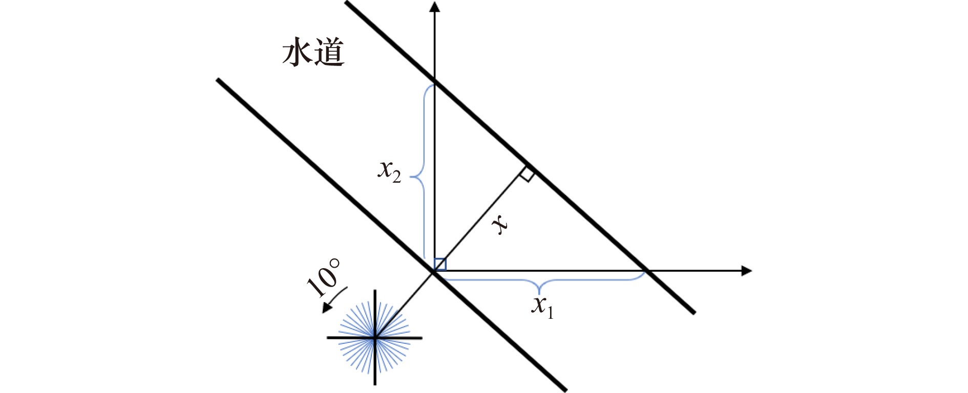
图 2 正交系下水道在两个方向的阔度与真实宽度的关系
Fig. 2 Relationship between lead extents and real lead width of an orthogonal system in two directions
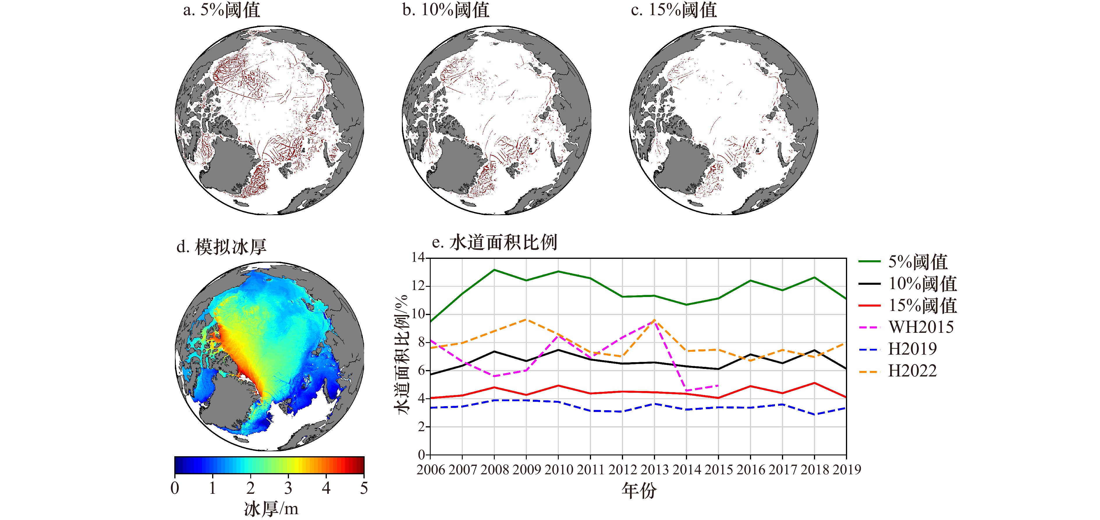
图 3 2009年1月4日不同阈值提取模拟水道结果(a、b、c),2009年1月4日模拟海冰厚度(d),2006年至2019年北极冬季(1月至4月)不同阈值方案提取的模拟水道面积比例和遥感产品的年际变化(e)
Fig. 3 Results of simulated lead extraction with different thresholds on 4 January 2009 (a, b, c), simulated sea ice thickness (d) on 4 January 2009, and interannual variation in the area fraction of simulated lead and remote sensing products extracted with different threshold schemes in Arctic winter (January to April) from 2006 to 2019 (e)
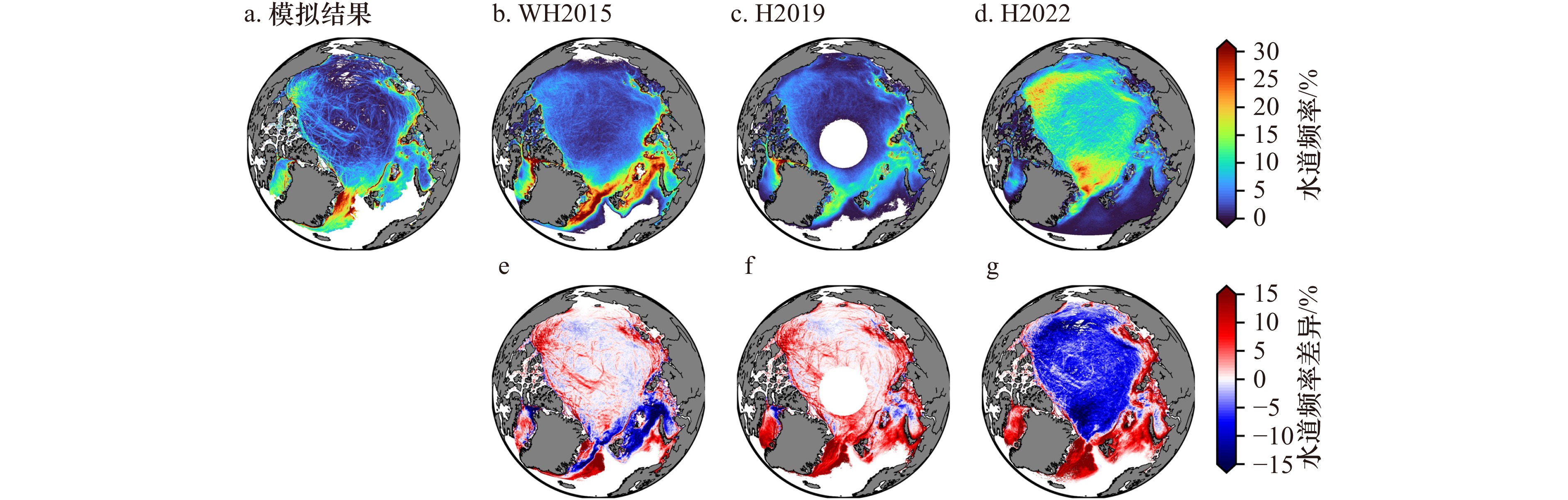
图 4 2009−2015年北极冬季模拟结果及3种卫星遥感产品冰间水道的出现频率与模拟结果减遥感产品的差值场
Fig. 4 The frequency of sea ice lead for simulation results and three satellite remote sensing products in the Arctic winter from 2009 to 2015 and difference field between simulation results and remote sensing products
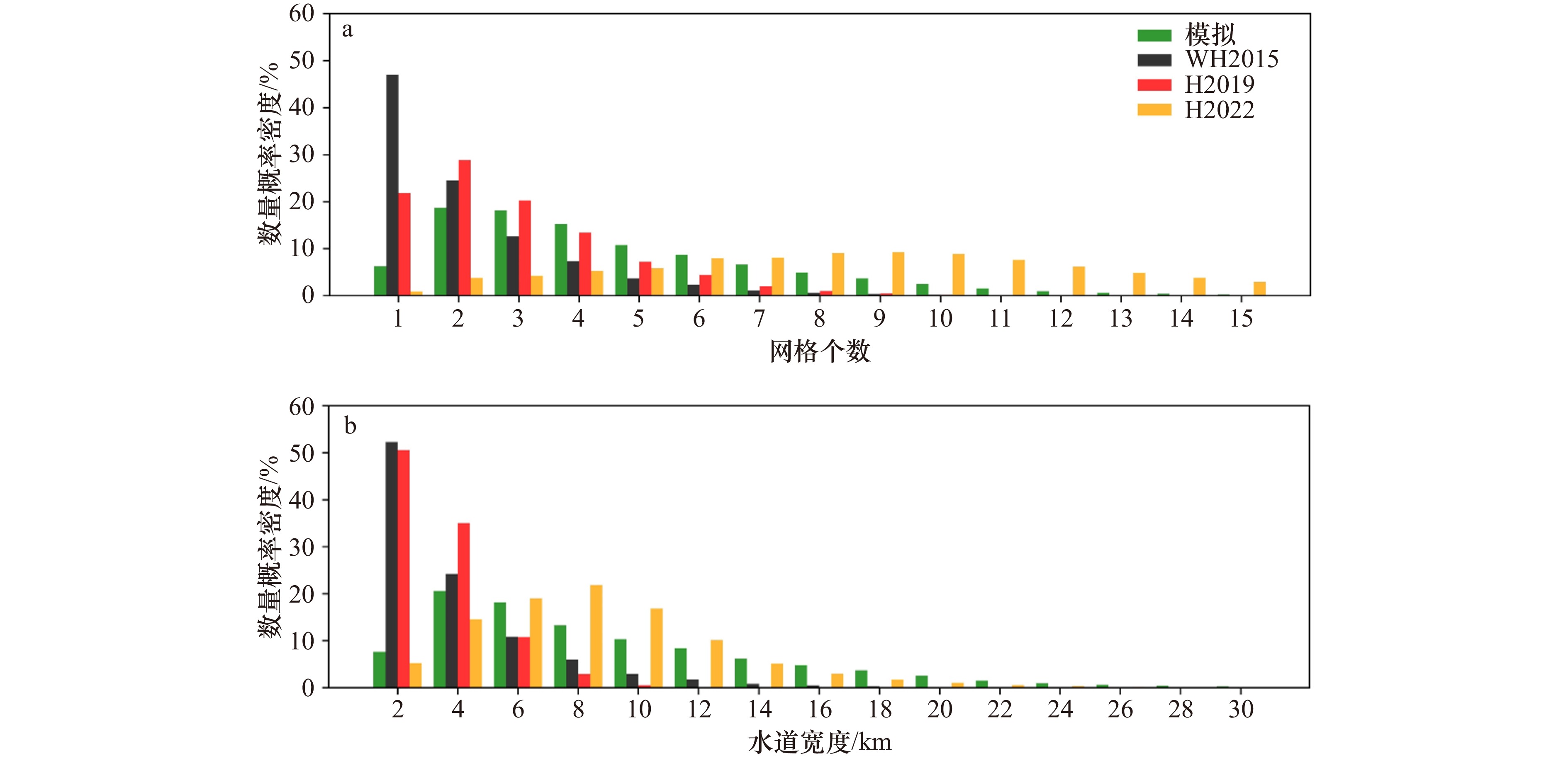
图 5 2006−2019年波弗特海冬季模拟结果及3种卫星遥感产品水道宽度的数量概率密度分布
a. 原始分辨率,b. 插值到2 km
Fig. 5 The quantity probability density distribution of winter lead width for simulation results and three satellite remote sensing products in Beaufort Sea from 2006 to 2019
a. Original resolution, b. interpolated to 2 km

图 6 2006−2019年波弗特海冬季模拟结果及3种卫星遥感产品水道平均宽度季节变化和年际变化(原始分辨率)
Fig. 6 The seasonal and interannual variations of the winter average lead width for simulation results and three satellite remote sensing products (original resolution)

图 7 2006−2019年波弗特海冬季模拟结果及3种卫星遥感产品冰间水道总长度季节和年际变化
a1−a6.原始分辨率各数据水道总长度,b1−b6.插值为2 km各数据水道总长度
Fig. 7 The seasonal and interannual variations of the winter lead total length for simulation results and three satellite remote sensing products
a1−a6. Represents the lead total length of each data at the original resolution, b1−b6. interpolates to 2 km for the lead total length of each data

图 8 2006−2019年波弗特海冬季模拟结果及3种卫星遥感产品各水道宽度的总长度分布
a. 原始分辨率,b. 插值到2 km
Fig. 8 The total length of winter lead of each width for simulation results and three satellite remote sensing products in Beaufort Sea from 2006 to 2019
a. Original resolution, b. interpolated to 2 km

图 9 波弗特海2006−2015年冰间水道走向年平均频率分布
Fig. 9 Annual average frequency distribution of lead orientation in the Beaufort Sea from 2006 to 2015

图 10 2009−2015年模拟结果及3种遥感产品的冰间水道平均走向
彩色线段代表水道数量,倾斜角度代表水道走向,宽度代表100 km × 100 km单元内水道走向的标准偏差,箭头代表平均冰速,红色代表水道和冰速方向夹角。a是模拟水道与模拟冰速夹角,b、c、d是遥感水道与遥感冰速夹角
Fig. 10 The average lead orientation of simulation results and three remote sensing products from 2009 to 2015
Colored line segments represent the number of leads, inclination angles represent the orientation of lead, width represents the standard deviation of lead orientation within a 100 km unit, arrows represent the average ice velocity, red represents the angle between lead and ice velocity in the direction. a. The angle between simulated lead and simulated ice velocity; b, c, d. the angle between remote sensing lead and remote sensing ice velocity
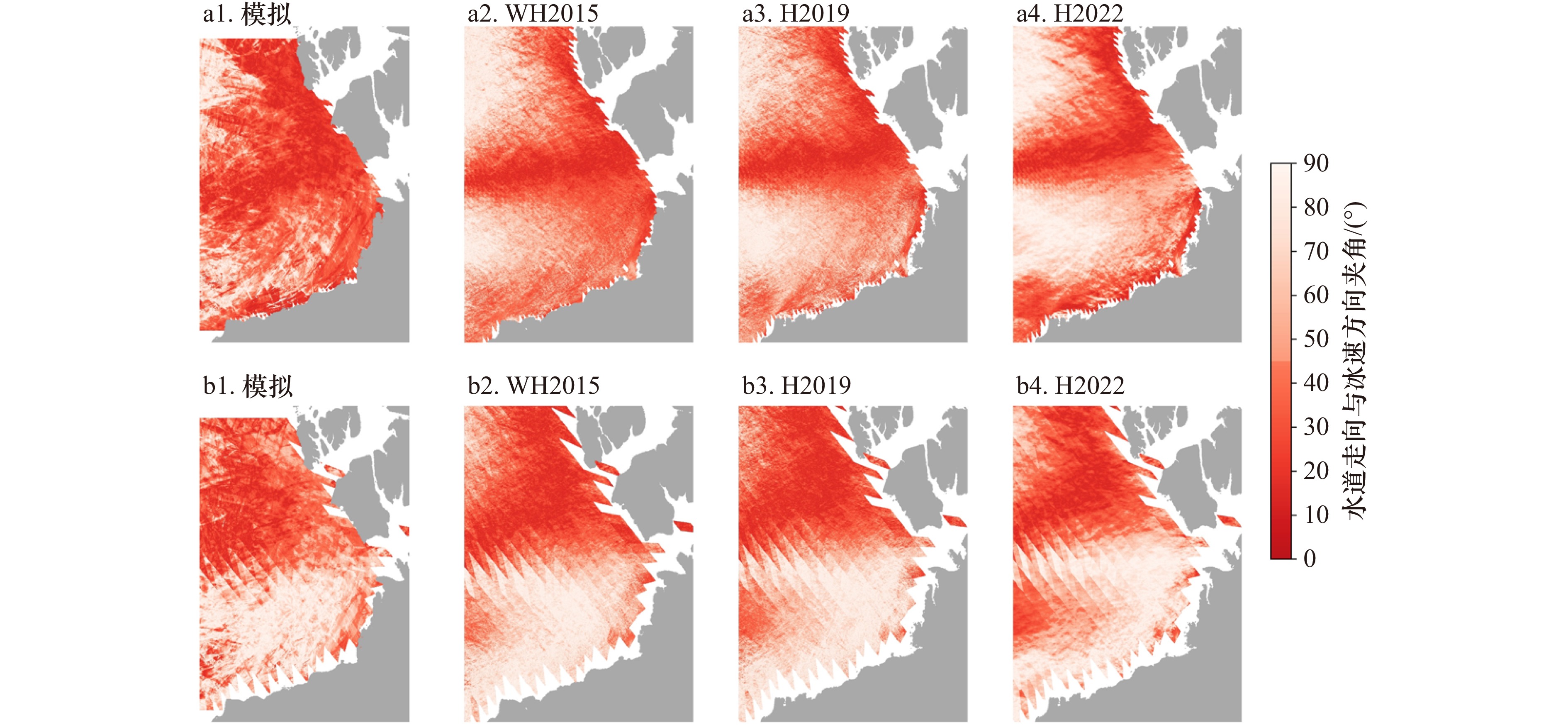
图 11 2010−2015年模拟结果与遥感产品水道走向与冰速方向夹角的空间分布
a1−a4. 水道走向与Pathfinder冰速数据夹角,b1−b4. 水道走向与OSISAF冰速数据夹角
Fig. 11 The spatial distribution of the angle between lead orientation and ice velocity direction for simulation results and the remote sensing products from 2010 to 2015
a1−a4. Represents the angle between the lead orientation and the Pathfinder ice velocity direction, b1−b4. represents the angle between the lead orientation and the OSISAF ice velocity direction
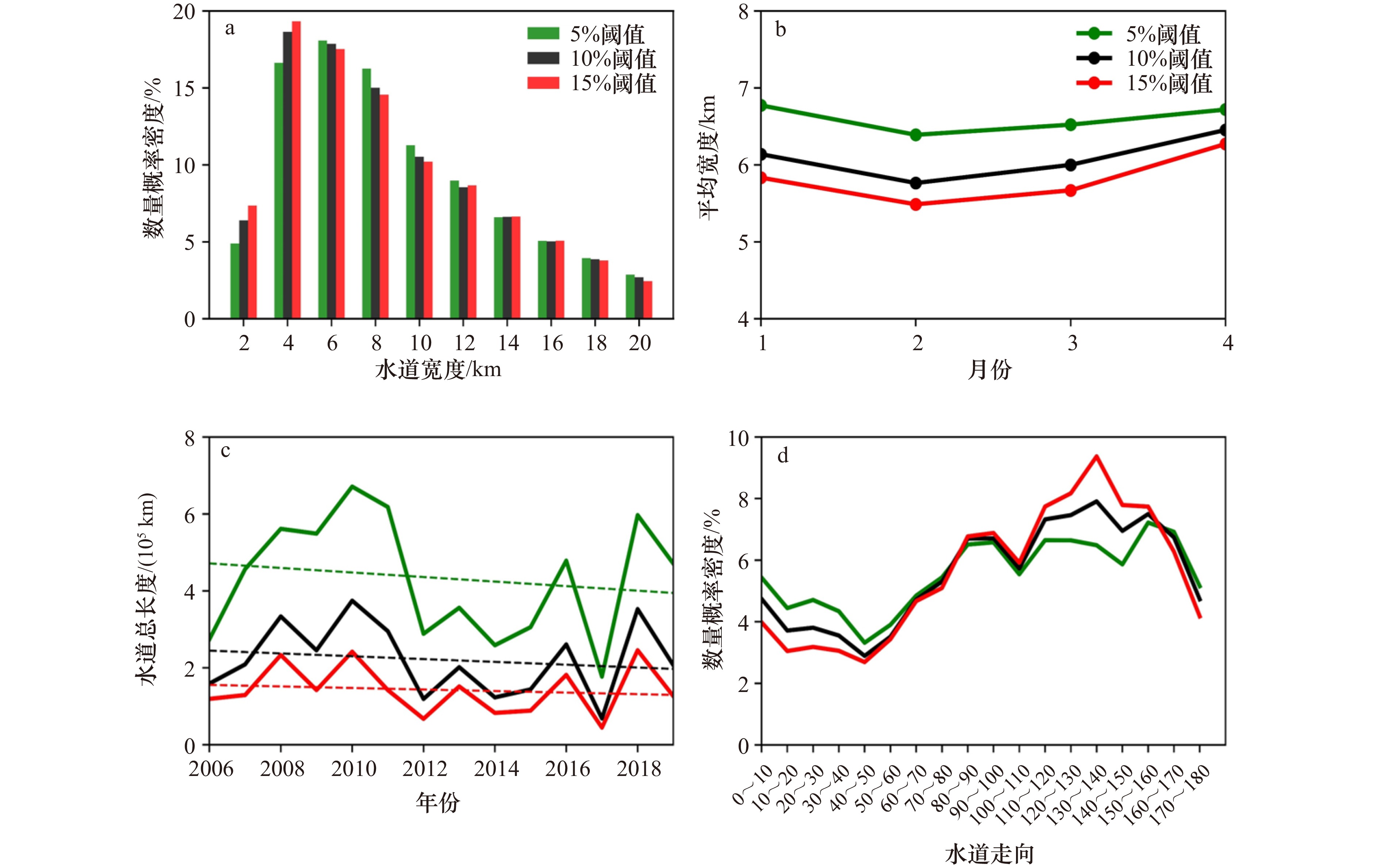
图 12 2006−2019年模拟冰厚场中不同阈值提取的水道形态分布特征
a. 水道宽度的数量概率密度分布,b. 水道平均宽度,c. 水道总长度,d. 水道走向
Fig. 12 Distribution characteristics of lead morphology extracted by different thresholds in simulated ice thickness fields from 2006 to 2019
a. Probability density distribution of lead width, b. average lead width, c. lead total length, d. lead orientation
表 1 模拟结果和遥感产品冰间水道幂律分布
$ \mathit{{N}}=mx^{-n} $ 的指数nTab. 1 The exponent n of the power-law distribution
${{N}} = m{x^{ - n}}$ of simulation results and remote sensing products for sea ice lead产品 冬季 月份 1 2 3 4 模拟 1.50 1.54 1.81 1.74 1.52 WH2015 1.57 1.64 1.67 1.64 1.51 H2019 1.43 1.46 1.45 1.43 1.43  下载: 导出CSV
表 2 2006−2019年模拟结果和遥感产品冰间水道平均宽度统计结果(单位:km)及相关系数
Tab. 2 The statistical results and correlation coefficients of average lead width (in kilometers) for simulation results and remote sensing products from 2006 to 2019 (in kilometers)
产品 评价指标 冬季 月份 1 2 3 4 模拟 平均 6.09 6.14 5.76 6.00 6.46 标准差 0.68 0.69 0.99 1.39 1.12 WH2015 平均 2.32 2.26 2.25 2.30 2.46 标准差 0.19 0.20 0.17 0.30 0.34 Pearson相关系数 0.58 0.54 0.15 0.75 0.15 H2019 平均 2.09 2.03 2.08 2.10 2.15 标准差 0.09 0.10 0.12 0.13 0.16 Pearson相关系数 0.34 0.33 0.29 0.25 0.10 H2022 平均 6.79 6.74 6.77 6.89 6.76 标准差 0.30 0.49 0.63 0.71 0.50 Pearson相关系数 0.07 −0.09 −0.02 0.47 −0.40
下载: 导出CSV
表 3 模拟结果和遥感产品水道总长度的Pearson相关系数矩阵
Tab. 3 Pearson correlation coefficient matrix of lead total length between simulation results and remote sensing product
月份 WH2015 H2019 H2022 1 0.42 0.50* 0.19 2 0.29 0.37 0.13 3 0.54 0.61* 0.46 4 0.43 0.13 −0.16 总计 0.34 0.33 −0.03 注:*,p < 0.05。
下载: 导出CSV
-
[1] Maykut G A. Large-scale heat exchange and ice production in the central Arctic[J]. Journal of Geophysical Research: Oceans, 1982, 87(C10): 7971−7984. doi: 10.1029/JC087iC10p07971 [2] Maykut G A. Energy exchange over young sea ice in the central Arctic[J]. Journal of Geophysical Research: Oceans, 1978, 83(C7): 3646−3658. doi: 10.1029/JC083iC07p03646 [3] Rampal P, Weiss J, Marsan D. Positive trend in the mean speed and deformation rate of Arctic sea ice, 1979−2007[J]. Journal of Geophysical Research: Oceans, 2009, 114(C5): C05013. [4] Alam A, Curry J A. Evolution of new ice and turbulent fluxes over freezing winter leads[J]. Journal of Geophysical Research: Oceans, 1998, 103(C8): 15783−15802. doi: 10.1029/98JC01188 [5] Maslanik J A, Key J. On treatments of fetch and stability sensitivity in large-area estimates of sensible heat flux over sea ice[J]. Journal of Geophysical Research: Oceans, 1995, 100(C3): 4573−4584. doi: 10.1029/94JC02204 [6] Bröhan D, Kaleschke L. A nine-year climatology of Arctic sea ice lead orientation and frequency from AMSR-E[J]. Remote Sensing, 2014, 6(2): 1451−1475. doi: 10.3390/rs6021451 [7] 屈猛. 北极波弗特海冰间水道的遥感提取及其热力学效应研究[D]. 武汉: 武汉大学, 2021.Qu Meng. Detection of sea ice leads in the Beaufort Sea using remote sensing imagery and estimation of energy budget over leads surface[D]. Wuhan: Wuhan University, 2021. [8] Lindsay R W, Rothrock D A. Arctic sea ice leads from advanced very high resolution radiometer images[J]. Journal of Geophysical Research: Oceans, 1995, 100(C3): 4533−4544. doi: 10.1029/94JC02393 [9] Hoffman J P, Ackerman S A, Liu Yinghui, et al. The detection and characterization of Arctic Sea ice leads with satellite imagers[J]. Remote Sensing, 2019, 11(5): 521. doi: 10.3390/rs11050521 [10] Willmes S, Heinemann G. Sea-ice wintertime lead frequencies and regional characteristics in the Arctic, 2003−2015[J]. Remote Sensing, 2016, 8(1): 4. [11] Qu Meng, Pang Xiaoping, Zhao Xi, et al. Spring leads in the Beaufort Sea and its interannual trend using Terra/MODIS thermal imagery[J]. Remote Sensing of Environment, 2021, 256: 112342. doi: 10.1016/j.rse.2021.112342 [12] Willmes S, Heinemann G. Pan-Arctic lead detection from MODIS thermal infrared imagery[J]. Annals of Glaciology, 2015, 56(69): 29−37. doi: 10.3189/2015AoG69A615 [13] Hoffman J P, Ackerman S A, Liu Yinghui, et al. Application of a convolutional neural network for the detection of sea ice leads[J]. Remote Sensing, 2021, 13(22): 4571. doi: 10.3390/rs13224571 [14] Hoffman J P, Ackerman S A, Liu Yinghui, et al. A 20-year climatology of sea ice leads detected in infrared satellite imagery using a convolutional neural network[J]. Remote Sensing, 2022, 14(22): 5763. doi: 10.3390/rs14225763 [15] Lindsay R W, Zhang Jinlun, Rothrock D A. Sea-ice deformation rates from satellite measurements and in a model[J]. Atmosphere-Ocean, 2003, 41(1): 35−47. doi: 10.3137/ao.410103 [16] Girard L, Weiss J, Molines J M, et al. Evaluation of high-resolution sea ice models on the basis of statistical and scaling properties of Arctic sea ice drift and deformation[J]. Journal of Geophysical Research: Oceans, 2009, 114(C8): C08015. [17] Hutter N, Losch M, Menemenlis D. Scaling properties of Arctic sea ice deformation in a high-resolution viscous-plastic sea ice model and in satellite observations[J]. Journal of Geophysical Research: Oceans, 2018, 123(1): 672−687. doi: 10.1002/2017JC013119 [18] Wang Qiang, Danilov S, Jung T, et al. Sea ice leads in the Arctic Ocean: model assessment, interannual variability and trends[J]. Geophysical Research Letters, 2016, 43(13): 7019−7027. doi: 10.1002/2016GL068696 [19] Bouillon S, Rampal P. Presentation of the dynamical core of neXtSIM, a new sea ice model[J]. Ocean Modelling, 2015, 91: 23−37. doi: 10.1016/j.ocemod.2015.04.005 [20] Dansereau V, Weiss J, Saramito P, et al. A Maxwell elasto-brittle rheology for sea ice modelling[J]. The Cryosphere, 2016, 10(3): 1339−1359. doi: 10.5194/tc-10-1339-2016 [21] Girard L, Bouillon S, Weiss J, et al. A new modeling framework for sea-ice mechanics based on elasto-brittle rheology[J]. Annals of Glaciology, 2011, 52(57): 123−132. doi: 10.3189/172756411795931499 [22] Hutter N, Zampieri L, Losch M. Leads and ridges in Arctic sea ice from RGPS data and a new tracking algorithm[J]. The Cryosphere, 2019, 13(2): 627−645. doi: 10.5194/tc-13-627-2019 [23] Hutter N, Losch M. Feature-based comparison of sea ice deformation in lead-permitting sea ice simulations[J]. The Cryosphere, 2020, 14(1): 93−113. doi: 10.5194/tc-14-93-2020 [24] Andreas E L, Murphy B. Bulk transfer coefficients for heat and momentum over leads and polynyas[J]. Journal of Physical Oceanography, 1986, 16(11): 1875−1883. doi: 10.1175/1520-0485(1986)016<1875:BTCFHA>2.0.CO;2 [25] Alam A, Curry J A. Determination of surface turbulent fluxes over leads in Arctic sea ice[J]. Journal of Geophysical Research: Oceans, 1997, 102(C2): 3331−3343. doi: 10.1029/96JC03606 [26] Marcq S, Weiss J. Influence of sea ice lead-width distribution on turbulent heat transfer between the ocean and the atmosphere[J]. The Cryosphere, 2012, 6(1): 143−156. doi: 10.5194/tc-6-143-2012 [27] Qu Meng, Pang Xiaoping, Zhao Xi, et al. Estimation of turbulent heat flux over leads using satellite thermal images[J]. The Cryosphere, 2019, 13(6): 1565−1582. doi: 10.5194/tc-13-1565-2019 [28] Losch M, Menemenlis D, Campin J M, et al. On the formulation of sea-ice models. Part 1: effects of different solver implementations and parameterizations[J]. Ocean Modelling, 2010, 33(1/2): 129−144. [29] Fraser A D, Massom R A, Michael K J. A method for compositing polar MODIS satellite images to remove cloud cover forlandfast sea-ice detection[J]. IEEE Transactions on Geoscience and Remote Sensing, 2009, 47(9): 3272−3282. doi: 10.1109/TGRS.2009.2019726 [30] Key J, Stone R, Maslanik J, et al. The detectability of sea-ice leads in satellite data as a function of atmospheric conditions and measurement scale[J]. Annals of Glaciology, 1993, 17: 227−232. doi: 10.3189/S026030550001288X [31] 屈猛, 赵羲, 庞小平, 等. 北极冰间水道区域的物理过程和遥感观测研究进展[J]. 地球科学进展, 2022, 37(4): 382−391. doi: 10.11867/j.issn.1001-8166.2021.102Qu Meng, Zhao Xi, Pang Xiaoping, et al. Review of Arctic sea ice leads: physics and remote sensing[J]. Advances in Earth Science, 2022, 37(4): 382−391. doi: 10.11867/j.issn.1001-8166.2021.102 [32] Beitsch A, Kaleschke L, Kern S. Investigating high-resolution AMSR2 sea ice concentrations during the February 2013 fracture event in the Beaufort Sea[J]. Remote Sensing, 2014, 6(5): 3841−3856. doi: 10.3390/rs6053841 [33] Schulson E M, Hibler W D. The fracture of ice on scales large and small: Arctic leads and wing cracks[J]. Journal of Glaciology, 1991, 37(127): 319−322. doi: 10.3189/S0022143000005748 -


计量
- 文章访问数: 388
- HTML全文浏览量: 145
- PDF下载量: 69
- 被引次数: 0
