中国东部海域浮游植物类群遥感反演研究

赵海阳; 沈芳; 孙雪融; 魏小岛

doi:10.12284/hyxb2022062

中国东部海域浮游植物类群遥感反演研究

doi: 10.12284/hyxb2022062

1.
华东师范大学河口海岸学国家重点实验室，上海 200241
2.
华东师范大学崇明生态研究院，上海 202162

基金项目: 国家自然科学基金（42076187，41771378）。

详细信息

作者简介:
赵海阳（1997-），男，河南省许昌市人，主要从事海洋水色遥感研究。E-mail: 51193904013@stu.ecnu.edu.cn

通讯作者:
沈芳，女，教授，主要从事海洋水色遥感研究。E-mail: fshen@sklec.ecnu.edu.cn

中图分类号: TP79
计量
- 文章访问数: 642
- HTML全文浏览量: 270
- PDF下载量: 85
- 被引次数: 0
出版历程
- 收稿日期: 2021-08-17
- 修回日期: 2021-11-20
- 刊出日期: 2022-04-14

Remote sensing retrieval of phytoplankton group in the eastern China seas

1.
State Key Laboratory of Estuarine and Coastal Research, East China Normal University, Shanghai 200241, China
2.
Institute of Eco-Chongming, East China Normal University, Shanghai 202162, China

摘要

摘要: 浮游植物类群遥感反演能够为全面认识浮游植物在海洋生态系统中的作用提供重要的数据资料。但由于复杂的水体光学特性，近海浮游植物类群遥感反演存在着巨大挑战。本研究以复杂光学二类水体—中国东部海域为研究区，通过使用3种建模方法，即波段组合法、基于奇异值分解的多元线性回归法、基于奇异值分解的XGBoost回归法，利用遥感反射率数据反演浮游植物类群。经原位实测数据集验证，基于奇异值分解的XGBoost回归法构建的8类浮游植物叶绿素a浓度反演模型的精度最高，其中硅藻、甲藻的叶绿素a浓度反演模型在验证集上的决定系数均大于0.7。相比之下，3种建模方法估算得到的绿藻、蓝藻和金藻的叶绿素a浓度精度较低（验证结果的决定系数小于0.45）。同时，研究评估了OLCI影像的3种大气校正方法（C2RCC、POLYMER、MUMM）在中国东部海域的适用性。结果显示，相对于其他两种大气校正算法，C2RCC在各波段有较好的表现（均方根误差小于0.004 8 sr⁻¹）。将3种浮游植物类群反演模型应用到大气校正后的OLCI影像，验证结果显示，利用基于奇异值分解的多元线性回归法建立的硅藻叶绿素a浓度模型有较好的反演精度（决定系数为0.56）。
- 中国东部海域 /
- 浮游植物类群 /
- 遥感反演 /
- OLCI /
- 大气校正
Abstract: Remote sensing retrieval of phytoplankton group can provide important data for a comprehensive understanding of the role of phytoplankton in marine ecosystem. However, due to the complex optical characteristics, there are still great challenges in the remote sensing retrieval of phytoplankton group in offshore waters. In this study, the eastern China seas region, a complex optical class II water body, is taken as the research area. By using three modeling methods, namely band combination method, multiple linear regression method based on singular value decomposition (SVD+MLR) and XGBoost regression method based on singular value decomposition (SVD+XGBoost), the phytoplankton group is retrieved from remote sensing reflectance (R_rs) data. Verified by the in-situ measured data set, the chlorophyll a (Chl a) concentration retrieval model of eight phytoplankton groups by SVD+XGBoost has the highest accuracy, and the determination coefficient (R²) of Chl a concentration inversion model of diatoms and dinoflagellates in the validation set is greater than 0.7. In contrast, the accuracy of Chl a concentration of chlorophytes, cyanobacteria and chrysophytes estimated by the three modeling methods is low (the R² of the validation results is less than 0.45). At the same time, the applicability of three atmospheric correction methods of OLCI images (C2RCC, POLYMER and MUMM) in the eastern China seas is evaluated. The results show that compared with the other two atmospheric correction algorithms, C2RCC has better performance in each band (root mean square error is less than 0.0048 sr⁻¹). Finally, the performance of the retrieval model on satellite images is verified by the in-situ data. The validation results show that the diatoms Chl a concentration model established by SVD+MLR has better accuracy (the R² is 0.56), while the Chl a concentration inversion models of other phytoplankton groups have poor results.
- eastern China seas /
- phytoplankton group /
- remote sensing retrieval /
- OLCI /
- atmospheric correction

HTML全文

图 1 研究区位置以及采样站位

Fig. 1 Location of the study area and sampling stations

下载: 全尺寸图片幻灯片

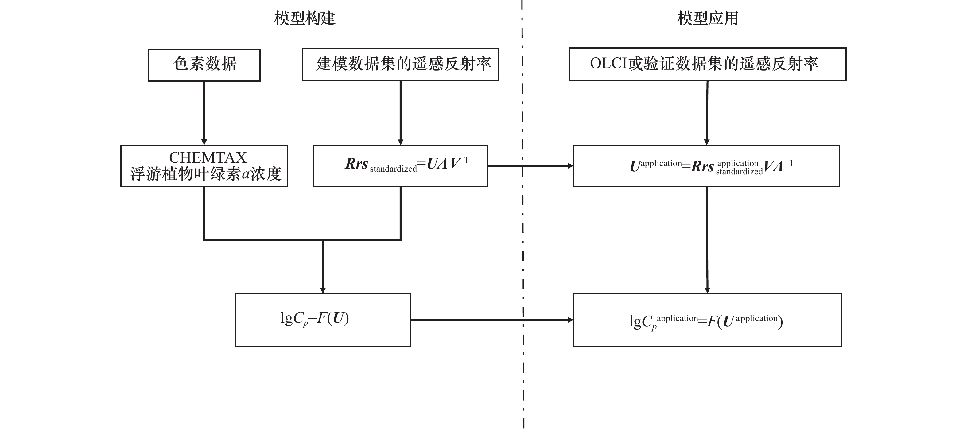
图 2 基于奇异值分解的浮游植物类群Chl a浓度反演算法流程

F表示本研究中使用的回归模型，即为多元线性回归模型或XGBoost回归模型

Fig. 2 Flow chart of Chl a concentration inversion algorithm of phytoplankton groups based on singular value decomposition

F represents the regression model used in this study, such as the multiple linear regression model or XGBoost regression model

下载: 全尺寸图片幻灯片

图 3 3种大气校正方法获得的遥感反射率与实测遥感反射率验证结果

Fig. 3 Validation of remote sensing reflectance obtained by three atmospheric correction methods with in-situ remote sensing reflectance

下载: 全尺寸图片幻灯片

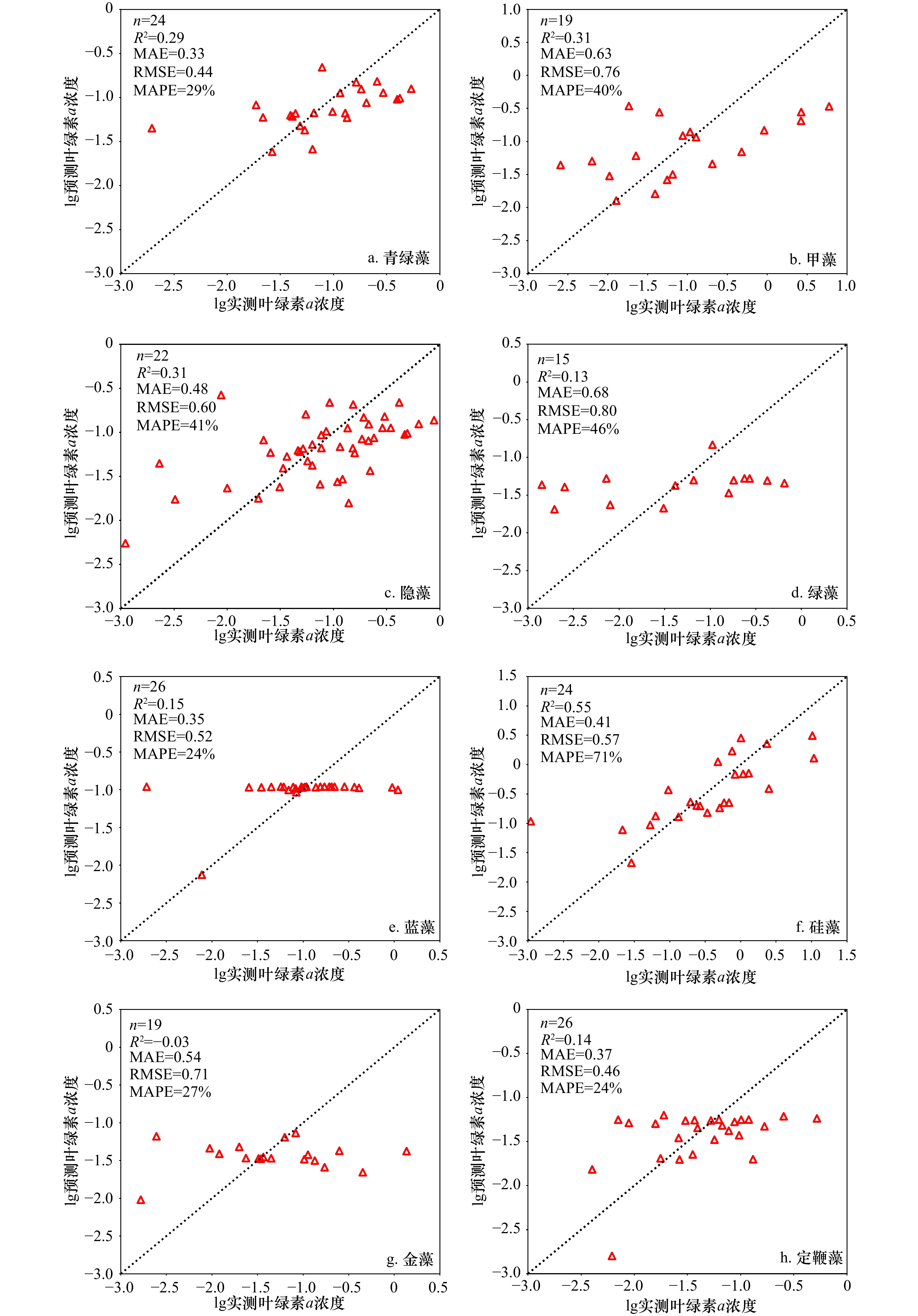
图 4 基于波段组合法建立的8类浮游植物叶绿素a浓度反演模型的验证结果（叶绿素a浓度单位：mg/m³）

Fig. 4 Validation results of Chl a concentration inversion model of eight phytoplankton groups based on band combination method (the unit of Chl a concentration is mg/m³)

下载: 全尺寸图片幻灯片

图 5 基于SVD+MLR建立的8类浮游植物叶绿素a浓度反演模型的验证结果（叶绿素a浓度单位：mg/m³）

Fig. 5 Validation results of Chl a concentration inversion model of eight phytoplankton groups based on SVD+MLR method (the unit of Chl a concentration is mg/m³)

下载: 全尺寸图片幻灯片

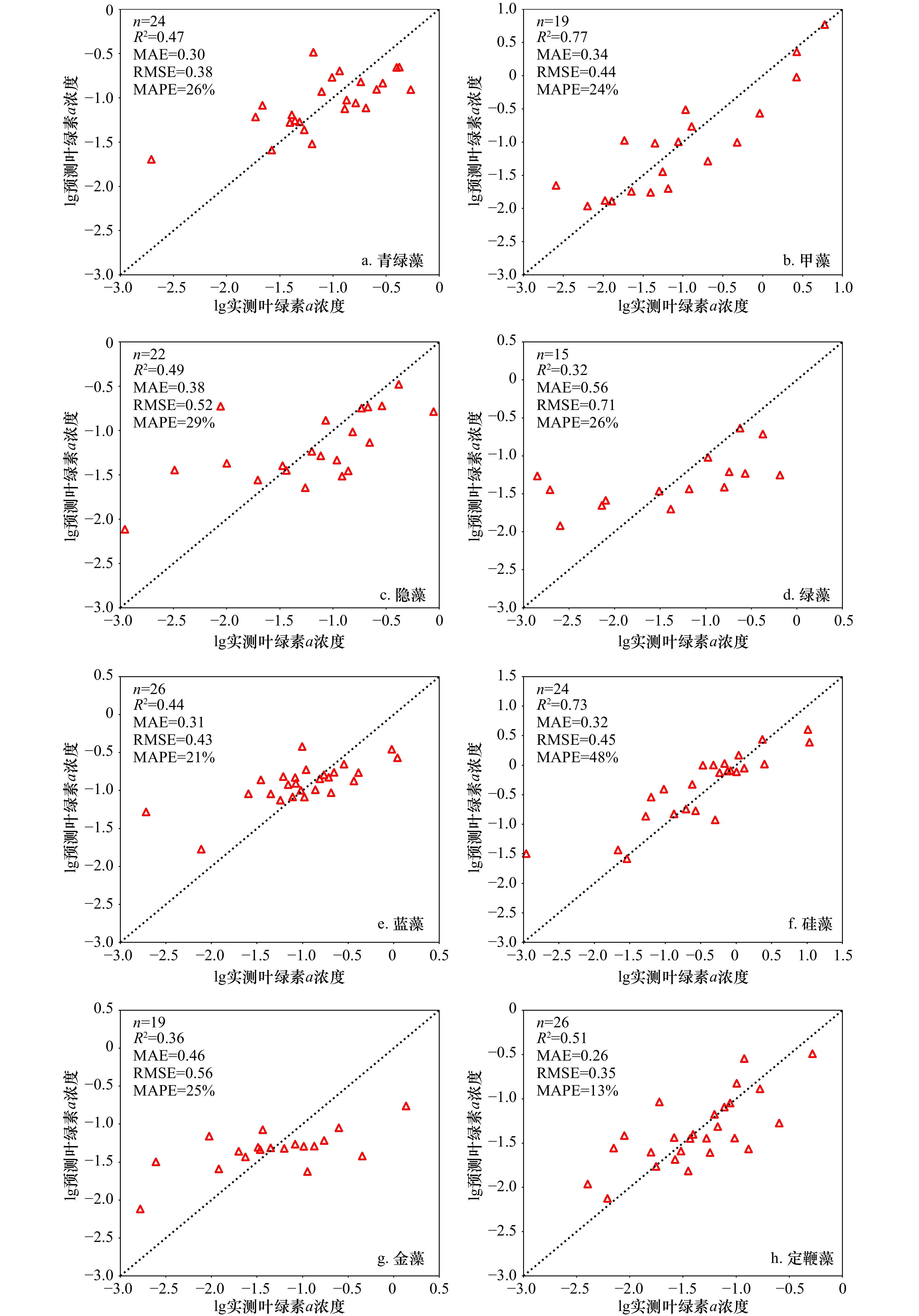
图 6 基于SVD+XGBoost建立的8类浮游植物叶绿素a浓度反演模型的验证结果（叶绿素a浓度单位：mg/m³）

Fig. 6 Validation results of Chl a concentration inversion model of eight phytoplankton groups based on SVD+XGBoost method (the unit of Chl a concentration is mg/m³)

下载: 全尺寸图片幻灯片

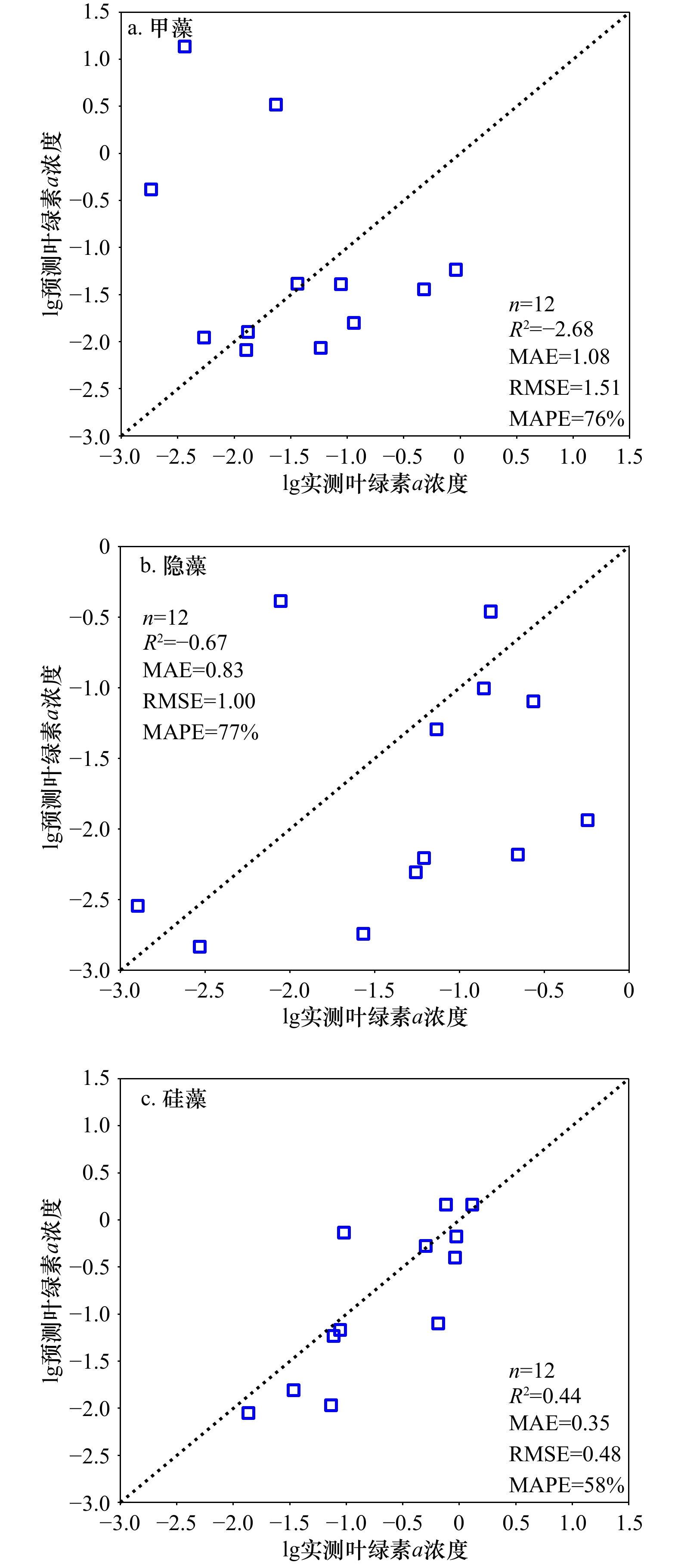
图 7 基于波段组合法的浮游植物类群叶绿素a浓度卫星反演验证（叶绿素a浓度单位：mg/m³）

Fig. 7 Validation of satellite inversion results of phytoplankton group Chl a concentration based on band combination method (the unit of Chl a concentration is mg/m³)

下载: 全尺寸图片幻灯片

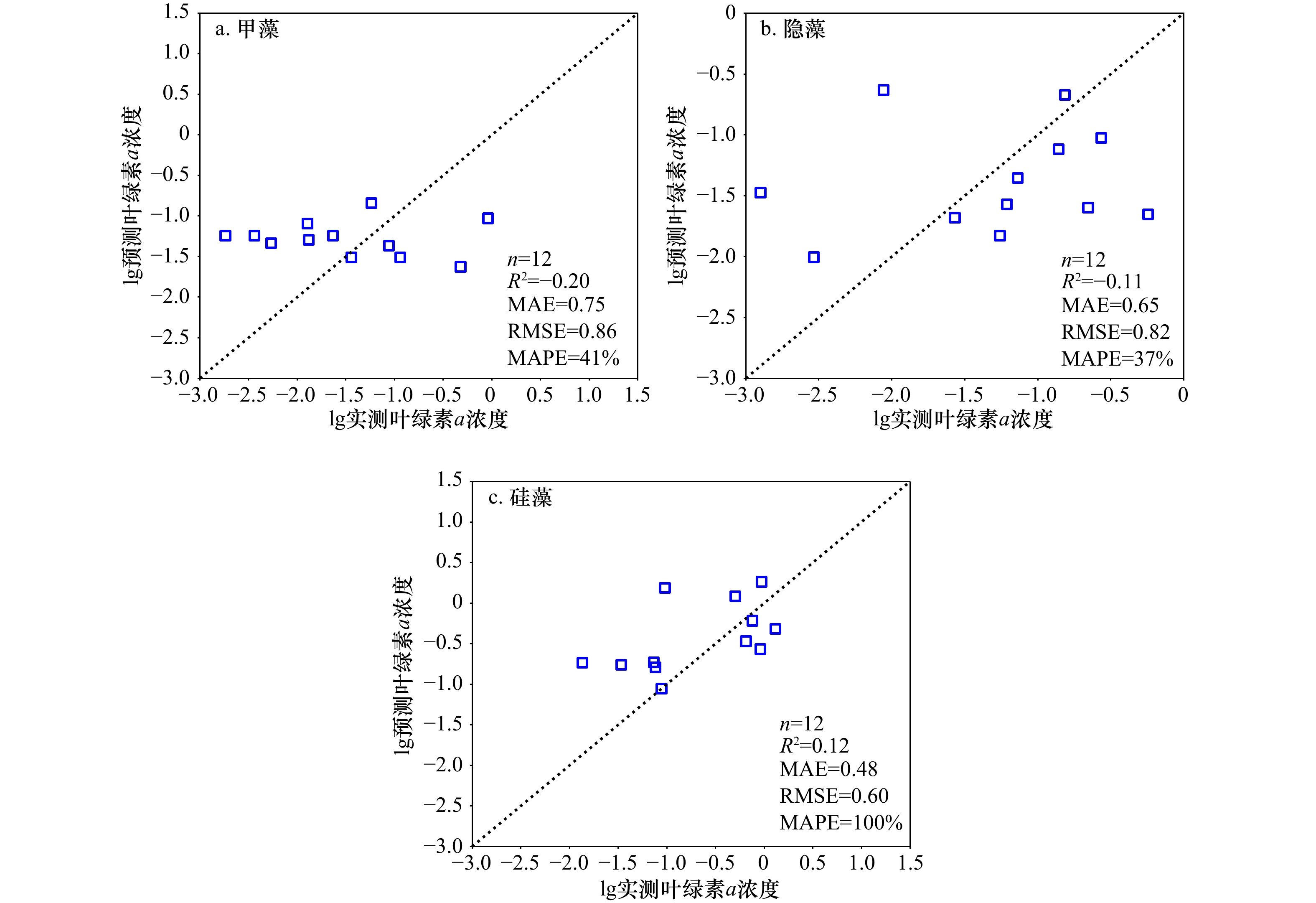
图 9 基于SVD+XGBoost的浮游植物类群叶绿素a浓度卫星反演验证（叶绿素a浓度单位：mg/m³）

Fig. 9 Validation of satellite inversion results of phytoplankton group Chl a concentration based on SVD+XGBoost method (the unit of Chl a concentration is mg/m³)

下载: 全尺寸图片幻灯片

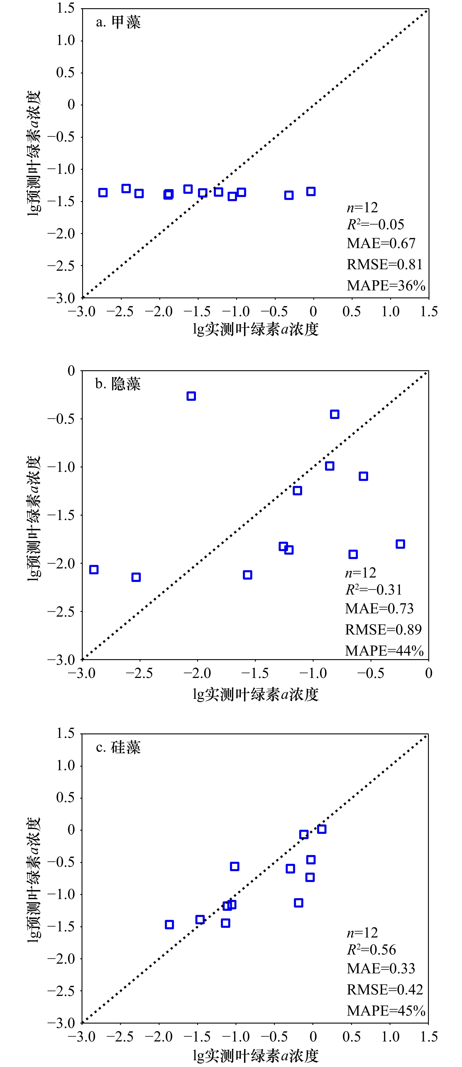
图 8 基于SVD+MLR的浮游植物类群叶绿素a浓度卫星反演验证（叶绿素a浓度单位：mg/m³）

Fig. 8 Validation of satellite inversion results of phytoplankton group Chl a concentration based on SVD+MLR method (the unit of Chl a concentration is mg/m³)

下载: 全尺寸图片幻灯片

图 10 2020年5月和2020年8月中国东部海域硅藻叶绿素a浓度空间分布

Fig. 10 The spatial distribution of diatom Chl a concentration in the eastern China seas in May 2020 and August 2020

下载: 全尺寸图片幻灯片

表 1 本研究采用的波段组合形式

Tab. 1 The band combinations used in this study

序号	波段（B）组合形式	序号	波段（B）组合形式
BC₁	$ {B}_{i}+{B}_{j} $	BC₆	$\dfrac{ {B}_{i}-{B}_{j} }{ {B}_{k} }$
BC₂	$ {B}_{i}-{B}_{j} $	BC₇	$\dfrac{ {B}_{i} }{ {B}_{j}+{B}_{k} }$
BC₃	$ {B}_{i}\times {B}_{j} $	BC₈	$\dfrac{ {B}_{i} }{ {B}_{j}-{B}_{k} }$
BC₄	$ {B}_{i}/{B}_{j} $	BC₉	${B}_{i}\times \left(\dfrac{1}{ {B}_{j} }+\dfrac{1}{ {B}_{k} }\right)$
BC₅	$\dfrac{ {B}_{i}+{B}_{j} }{ {B}_{k} }$	BC₁₀	${B}_{i}\times \left(\dfrac{1}{ {B}_{j} }-\dfrac{1}{ {B}_{k} }\right)$

下载: 导出CSV

表 2 8类浮游植物叶绿素a浓度统计特征

Tab. 2 Statistical characteristics of Chl a concentration of eight phytoplankton groups

浮游植物	站位数（N）	平均值/ （mg∙m⁻³）	标准差/ （mg∙m⁻³）	最大值/ （mg∙m⁻³）
青绿藻	450	0.15	0.27	4.45
甲藻	380	0.29	0.89	10.91
隐藻	410	0.17	0.22	1.31
绿藻	216	0.22	0.77	7.45
蓝藻	465	0.24	0.68	9.85
硅藻	446	1.13	2.10	15.23
金藻	360	0.11	0.23	2.51
定鞭藻	458	0.08	0.14	1.74

下载: 导出CSV

表 3 3种大气校正算法的精度评价

Tab. 3 Accuracy evaluation of three atmospheric correction algorithms

波长/nm	RMSE/（10⁻³ sr⁻¹）			MAE/（10⁻³ sr⁻¹）			MAPE/%
波长/nm	C2RCC	POLYMER	MUMM	C2RCC	POLYMER	MUMM	C2RCC	POLYMER	MUMM
400	4.13	4.41	10.79	3.21	3.67	9.83	41	44	213
412.5	3.99	4.36	7.68	3.01	3.53	6.69	36	41	141
442.5	4.10	4.64	6.81	3.21	3.68	6.02	36	39	140
490	4.79	4.97	4.90	3.74	3.82	4.43	40	37	89
510	4.72	5.28	4.21	3.65	4.12	3.74	40	41	70
560	4.34	5.31	3.53	3.31	4.03	3.04	33	43	56
620	3.22	4.21	3.05	2.24	3.21	2.44	49	66	81
665	3.21	3.75	2.71	2.21	2.82	2.05	61	72	84
673.75	3.23	3.64	2.62	2.29	2.72	1.98	63	71	80
681.25	3.21	3.64	2.60	2.29	2.75	1.91	64	73	83
708.75	3.12	4.45	3.21	2.21	3.62	1.93	70	116	69
753.75	3.21	3.24	2.38	2.30	2.40	1.49	88	94	81
778.75	3.04	3.23	2.40	2.18	2.40	1.44	86	99	90

下载: 导出CSV

表 4 8类浮游植物叶绿素a浓度反演模型使用的波段组合形式及回归方程

Tab. 4 Band combinations form and regression equations used in Chl a concentration inversion model of eight phytoplankton groups

浮游植物	波段组合	与Chl a浓度对数的相关系数	回归方程
青绿藻	${X=\dfrac{ {R}_{{\rm{rs}}}\left(442.5\right)+{R}_{{\rm{rs}}}\left(620\right)}{ {R}_{{\rm{rs}}}\left(560\right)}}$	0.53	${ \mathrm{l}\mathrm{g}C_P=-0.74X+0.09 }$
甲藻	${X=\dfrac{ {R}_{{\rm{rs}}}\left(442.5\right)}{ {R}_{{\rm{rs}}}\left(510\right)}-\dfrac{ {R}_{{\rm{rs}}}\left(442.5\right)}{ {R}_{{\rm{rs}}}\left(560\right)}}$	0.54	${ \mathrm{l}\mathrm{g}C_P=-7.83{X}^{3}-0.21{X}^{2}+3.97X-1.05 }$
隐藻	${X=\dfrac{ {R}_{{\rm{rs}}}\left(442.5\right)+{R}_{{\rm{rs}}}\left(490\right)}{ {R}_{{\rm{rs}}}\left(510\right)}}$	0.61	${ \mathrm{l}\mathrm{g}C_P=-2.10X+2.87} $
绿藻	${X=\dfrac{ {R}_{{\rm{rs}}}\left(560\right)}{ {R}_{{\rm{rs}}}\left(442.5\right)-{R}_{{\rm{rs}}}\left(620\right)}}$	0.37	${ \mathrm{l}\mathrm{g}C_P=2.2\times 1{0}^{-4}{X}^{2}-3.8\times {10}^{-2}{X}-1.25 }$
蓝藻	${X=\dfrac{ {R}_{{\rm{rs}}}\left(412.5\right)}{ {R}_{{\rm{rs}}}\left(442.5\right)-{R}_{{\rm{rs}}}\left(620\right)}}$	0.40	${ \mathrm{l}\mathrm{g}C_P=-0.006X-0.951 }$
硅藻	${X=\dfrac{ {R}_{{\rm{rs}}}\left(490\right)+{R}_{{\rm{rs}}}\left(620\right)}{ {R}_{{\rm{rs}}}\left(560\right)}}$	0.76	$ {\mathrm{l}\mathrm{g}C_P=-1.93X+2.75} $
金藻	$ {X={R}_{{\rm{rs}}}\left(665\right)-{R}_{{\rm{rs}}}\left(673.75\right) }$	0.34	${ \mathrm{l}\mathrm{g}C_P=-477\;853.92{X}^{2}-1\;569.03X-1.46 }$
定鞭藻	${X=\dfrac{ {R}_{{\rm{rs}}}\left(490\right)-{R}_{{\rm{rs}}}\left(510\right)}{ {R}_{{\rm{rs}}}\left(560\right)}}$	0.42	${ \mathrm{l}\mathrm{g}C_P=-2.143X-1.285} $

下载: 导出CSV

表 5 8类浮游植物叶绿素a浓度遥感反演模型的精度评价

Tab. 5 Accuracy of inversion model for Chl a concentration of eight phytoplankton groups

浮游植物类群	建模方法	R²	MAE	RMSE	MAPE/%
青绿藻	BC	0.29	0.33	0.44	29
	SVD+MLR	0.38	0.33	0.42	33
	SVD+XGBoost	0.47	0.30	0.38	26
甲藻	BC	0.31	0.63	0.76	40
	SVD+MLR	0.42	0.62	0.69	52
	SVD+XGBoost	0.77	0.34	0.44	24
隐藻	BC	0.31	0.48	0.60	41
	SVD+MLR	0.43	0.42	0.55	25
	SVD+XGBoost	0.49	0.38	0.52	29
绿藻	BC	0.13	0.68	0.80	46
	SVD+MLR	−0.06	0.77	0.89	56
	SVD+XGBoost	0.32	0.56	0.71	26
蓝藻	BC	0.15	0.35	0.52	24
	SVD+MLR	0.06	0.39	0.55	29
	SVD+XGBoost	0.44	0.31	0.43	21
硅藻	BC	0.55	0.41	0.57	71
	SVD+MLR	0.64	0.39	0.52	63
	SVD+XGBoost	0.73	0.32	0.45	48
金藻	BC	−0.03	0.54	0.71	27
	SVD+MLR	0.06	0.52	0.68	27
	SVD+XGBoost	0.36	0.46	0.56	25
定鞭藻	BC	0.14	0.37	0.46	24
	SVD+MLR	0.37	0.32	0.40	20
	SVD+XGBoost	0.51	0.26	0.35	13

下载: 导出CSV

参考文献(49)

[1]	Field C B, Behrenfeld M J, Randerson J T,et al. Primary production of the biosphere: integrating terrestrial and oceanic components[J]. Science, 1998, 281(5374): 237−240. doi: 10.1126/science.281.5374.237
[2]	Behrenfeld M J. Climate-mediated dance of the plankton[J]. Nature Climate Change, 2014, 4(10): 880−887. doi: 10.1038/nclimate2349
[3]	Le Quéré C, Harrison S P, Prentice I C, et al. Ecosystem dynamics based on plankton functional types for global ocean biogeochemistry models[J]. Global Change Biology, 2005, 11(11): 2016−2040.
[4]	Tréguer P, Bowler C, Moriceau B, et al. Influence of diatom diversity on the ocean biological carbon pump[J]. Nature Geoscience, 2018, 11(1): 27−37. doi: 10.1038/s41561-017-0028-x
[5]	Nair A, Sathyendranath S, Platt T, et al. Remote sensing of phytoplankton functional types[J]. Remote Sensing of Environment, 2008, 112(8): 3366−3375. doi: 10.1016/j.rse.2008.01.021
[6]	McClain C R. A decade of satellite ocean color observations[J]. Annual Review of Marine Science, 2009, 1(1): 19−42. doi: 10.1146/annurev.marine.010908.163650
[7]	Tilstone G H, Pardo S, Dall’Olmo G, et al. Performance of ocean colour Chlorophyll a algorithms for Sentinel-3 OLCI, MODIS-Aqua and Suomi-VIIRS in open-ocean waters of the Atlantic[J]. Remote Sensing of Environment, 2021, 260: 112444. doi: 10.1016/j.rse.2021.112444
[8]	Kostadinov T S, Cabré A, Vedantham H, et al. Inter-comparison of phytoplankton functional type phenology metrics derived from ocean color algorithms and Earth System Models[J]. Remote Sensing of Environment, 2017, 190: 162−177. doi: 10.1016/j.rse.2016.11.014
[9]	Bracher A, Bouman H A, Brewin R J W, et al. Obtaining phytoplankton diversity from ocean color: A scientific roadmap for future development[J]. Frontiers in Marine Science, 2017, 4: 55.
[10]	IOCCG. Phytoplankton functional types from space[R]. Dartmouth: International Ocean-Colour Coordinating Group, 2014.
[11]	Mouw C B, Hardman-Mountford N J, Alvain S, et al. A consumer’s guide to satellite remote sensing of multiple phytoplankton groups in the global ocean[J]. Frontiers in Marine Science, 2017, 4: 41.
[12]	Sun Xuerong, Shen Fang, Liu Dongyan, et al. In situ and satellite observations of phytoplankton size classes in the entire Continental Shelf Sea, China[J]. Journal of Geophysical Research: Oceans, 2018, 123(5): 3523−3544. doi: 10.1029/2017JC013651
[13]	李楠, 孙德勇, 环宇, 等. 黄渤海浮游植物种群比吸收光谱的确定及其应用[J]. 光学学报, 2020, 40(6): 060100. Li Nan, Sun Deyong, Huan Yu, et al. Determination and application of specific absorption spectra of phytoplankton species in Yellow Sea and Bohai Sea[J]. Acta Optica Sinica, 2020, 40(6): 060100.
[14]	O'Reilly J E, Maritorena S, Mitchell B G, et al. Ocean color chlorophyll algorithms for SeaWiFS[J]. Journal of Geophysical Research:Oceans, 1998, 103(C11): 24937−24953. doi: 10.1029/98JC02160
[15]	Hu Chuanmin, Lee Z, Franz B. Chlorophyll a algorithms for oligotrophic oceans: A novel approach based on three-band reflectance difference[J]. Journal of Geophysical Research: Oceans, 2012, 117(C1): C010011.
[16]	Xi Hongyan, Losa S N, Mangin A, et al. Global retrieval of phytoplankton functional types based on empirical orthogonal functions using CMEMS GlobColour merged products and further extension to OLCI data[J]. Remote Sensing of Environment, 2020, 240: 111704. doi: 10.1016/j.rse.2020.111704
[17]	Bracher A, Xi Hongyan, Dinter T, et al. High resolution water column phytoplankton composition across the Atlantic Ocean from ship-towed vertical undulating radiometry[J]. Frontiers in Marine Science, 2020, 7: 235. doi: 10.3389/fmars.2020.00235
[18]	Cao Zhigang, Ma Ronghua, Duan Hongtao, et al. A machine learning approach to estimate chlorophyll-a from Landsat-8 measurements in inland lakes[J]. Remote Sensing of Environment, 2020, 248: 111974. doi: 10.1016/j.rse.2020.111974
[19]	Liu Huizeng, Li Qingquan, Bai Yan, et al. Improving satellite retrieval of oceanic particulate organic carbon concentrations using machine learning methods[J]. Remote Sensing of Environment, 2021, 256: 112316. doi: 10.1016/j.rse.2021.112316
[20]	Kyryliuk D, Kratzer S. Evaluation of Sentinel-3A OLCI products derived using the case-2 regional coastcolour processor over the Baltic Sea[J]. Sensors, 2019, 19(16): 3609. doi: 10.3390/s19163609
[21]	He X Q, Bai Yan, Pan Delu. , et al. Satellite views of the seasonal and interannual variability of phytoplankton blooms in the eastern China seas over the past 14 yr (1998–2011)[J]. Biogeosciences, 2013, 10(7): 4721−4739. doi: 10.5194/bg-10-4721-2013
[22]	宋金明. 中国近海生态系统碳循环与生物固碳[J]. 中国水产科学, 2011, 18(3): 703−711. Song Jinming. Carbon cycling processes and carbon fixed by organisms in China marginal seas[J]. Journal of Fishery Sciences of China, 2011, 18(3): 703−711.
[23]	陈建忠, 葛建忠, Richard B. 东海中部浮游生态系统季节变化的数值模拟[J]. 华东师范大学学报(自然科学版), 2019(6): 153−168. Chen Jianzhong, Ge Jianzhong, Richard B. Numerical simulation of pelagic ecosystem’s seasonal variation in the central East China Sea[J]. Journal of East China Normal University (Natural Science), 2019(6): 153−168.
[24]	黄邦钦, 肖武鹏, 柳欣. 中国边缘海浮游植物群落时空格局与演变趋势[J]. 厦门大学学报(自然科学版), 2021, 60(2): 390−397. Huang Bangqin, Xiao Wupeng, Liu Xin. Spatial-temporal distributions and successional patterns of phytoplankton communities in the Chinese marginal seas[J]. Journal of Xiamen University (Natural Science), 2021, 60(2): 390−397.
[25]	Sokoletsky L G, Shen Fang. Optical closure for remote-sensing reflectance based on accurate radiative transfer approximations: the case of the Changjiang (Yangtze) River Estuary and its adjacent coastal area, China[J]. International Journal of Remote Sensing, 2014, 35(11/12): 4193−4224.
[26]	Zhang H K, Roy D P, Yan Lin, et al. Characterization of Sentinel-2A and Landsat-8 top of atmosphere, surface, and nadir BRDF adjusted reflectance and NDVI differences[J]. Remote Sensing of Environment, 2018, 215: 482−494. doi: 10.1016/j.rse.2018.04.031
[27]	Catlett D, Siegel D A. Phytoplankton pigment communities can be modeled using unique relationships with spectral absorption signatures in a dynamic coastal environment[J]. Journal of Geophysical Research: Oceans, 2018, 123(1): 246−264. doi: 10.1002/2017JC013195
[28]	Sun Xuerong, Shen Fang, Brewin Robert J W, et al. Twenty-year variations in satellite-derived chlorophyll a and phytoplankton size in the Bohai Sea and Yellow Sea[J]. Journal of Geophysical Research: Oceans, 2019, 124(12): 8887−8912. doi: 10.1029/2019JC015552
[29]	孙雪融. 东中国海浮游植物粒级结构定量遥感研究[D]. 上海: 华东师范大学, 2021 Sun Xuerong. Remote sensing quantitative retrieval of phytoplankton size classes in eastern China seas[D]. Shanghai: East China Normal University, 2021.
[30]	Mackey M D, Mackey D J, Higgins H W, et al. CHEMTAX—A program for estimating class abundances from chemical markers: Application to HPLC measurements of phytoplankton[J]. Marine Ecology Progress Series, 1996, 144(1/3): 265−283.
[31]	Sun Deyong, Lai Wendian, Wang Shengqiang, et al. Synoptic relationships to estimate phytoplankton communities specific to sizes and species from satellite observations in coastal waters[J]. Optics Express, 2019, 27(16): A1156−A1172. doi: 10.1364/OE.27.0A1156
[32]	Donlon C, Berruti B, Buongiorno A, et al. The global monitoring for environment and security (GMES) Sentinel-3 mission[J]. Remote Sensing of Environment, 2012, 120: 37−57. doi: 10.1016/j.rse.2011.07.024
[33]	Brockmann C, Doerffer R, Peters M, et al. Evolution of the C2RCC neural network for sentinel 2 and 3 for the retrieval of ocean colour products in normal and extreme optically complex waters[C]// Proceedings of the Living Planet Symposium, [S.l.]: [s.n.], 2016.
[34]	Doerffer R. , Schiller H. The MERIS Case 2 water algorithm[J]. International Journal of Remote Sensing, 2007, 28(3/4): 517−535.
[35]	Steinmetz F, Deschamps P Y, Ramon D. Atmospheric correction in presence of sun glint: application to MERIS[J]. Optics Express, 2011, 19(10): 9783−9800. doi: 10.1364/OE.19.009783
[36]	Steinmetz F, Ramon D. Sentinel-2 MSI and Sentinel-3 OLCI consistent ocean colour products using POLYMER[C]// Proceedings of SPIE 10778 Remote Sensing of the Open and Coastal Ocean and Inland Waters. Washington: SPIE, 2018: 107780E.
[37]	Gordon H R, Wang Menghua. Retrieval of water-leaving radiance and aerosol optical thickness over the oceans with SeaWiFS: a preliminary algorithm[J]. Applied Optics, 1994, 33(3): 443−452. doi: 10.1364/AO.33.000443
[38]	Ruddick K G, Ovidio F, Rijkeboer M. Atmospheric correction of SeaWiFS imagery for turbid coastal and inland waters[J]. Applied Optics, 2000, 39(6): 897−912. doi: 10.1364/AO.39.000897
[39]	Chen Tianqi, Guestrin C. XGBoost: A Scalable Tree Boosting System[C]// Proceedings of the 22nd ACM SIGKDD International Conference on Knowledge Discovery and Data Mining. California: Association for Computing Machinery, 2016: 785−794.
[40]	Tu Qianguang, Hao Zengzhou, Yan Yunwei, et al. Aerosol optical properties around the East China Seas based on AERONET measurements[J]. Atmosphere, 2021, 12(5): 642. doi: 10.3390/atmos12050642
[41]	Zagolski F, Santer R, Aznay O. A new climatology for atmospheric correction based on the aerosol inherent optical properties[J]. Journal of Geophysical Research: Atmospheres, 2007, 112(D14): D14208. doi: 10.1029/2006JD007496
[42]	Ahmad Z, Franz B A, McClain C R, et al. New aerosol models for the retrieval of aerosol optical thickness and normalized water-leaving radiances from the SeaWiFS and MODIS sensors over coastal regions and open oceans[J]. Applied Optics, 2010, 49(29): 5545−5560. doi: 10.1364/AO.49.005545
[43]	Wang Dian, Ma Ronghua, Xue Kun, et al. The assessment of Landsat-8 OLI atmospheric correction algorithms for inland waters[J]. Remote Sensing, 2019, 11(2): 169. doi: 10.3390/rs11020169
[44]	Shen Ming, Duan Hongtao, Cao Zhigang, et al. Sentinel-3 OLCI observations of water clarity in large lakes in eastern China: Implications for SDG 6.3. 2 evaluation[J]. Remote Sensing of Environment, 2020, 247: 111950. doi: 10.1016/j.rse.2020.111950
[45]	Doron M, Bélanger S, Doxaran D, et al. Spectral variations in the near-infrared ocean reflectance[J]. Remote Sensing of Environment, 2011, 115(7): 1617−1631. doi: 10.1016/j.rse.2011.01.015
[46]	自然资源部海洋预警监测司. 2020中国海洋灾害公报[R]. 北京: 自然资源部海洋预警监测司, 2021 Department of Marine Early Warning and Monitoring Ministry of Natural Resources. Bulletin of China marine disater, 2020[R]. Beijing: Department of Marine Early Warning and Monitoring, Ministry of Natural Resources, 2021.
[47]	江杉, 王益澄, 马仁锋. 中国东海叶绿素浓度变化分析及其海水温度响应[J]. 测绘通报, 2020(6): 39−44. Jiang Shan, Wang Yicheng, Ma Renfeng. Change conalysis of chlorophyll concentration in the East China Sea and its response to seawater temperature[J]. Bulletin of Surveying and Mapping, 2020(6): 39−44.
[48]	陈楠生, 陈阳. 中国海洋浮游植物和赤潮物种的生物多样性研究进展(二): 东海[J]. 海洋与湖沼, 2021, 52(2): 363-38. Chen Nansheng, Chen Yang. Advances in the study of biodiversity of phytoplankton and red tide species in China (II): the East China Sea[J]. Oceanologia et Limnologia Sinica, 2021, 52(2): 363−384.
[49]	田洪阵, 刘沁萍, Goes J I, 等. 基于2002−2018年MODIS数据的黄海叶绿素a时空变化研究[J]. 海洋通报, 2020, 39(1): 101−110. Tian Hongzhen, Liu Qinping, Goes J I, et al. Temporal and spatial changes in chlorophyll a concentrations in the Yellow Sea from 2002 to 2018 based on MODIS data[J]. Marine Science Bulletin, 2020, 39(1): 101−110.