

Test of salinity profile correction method for MVP system based on temperature gradient profile analysis
-
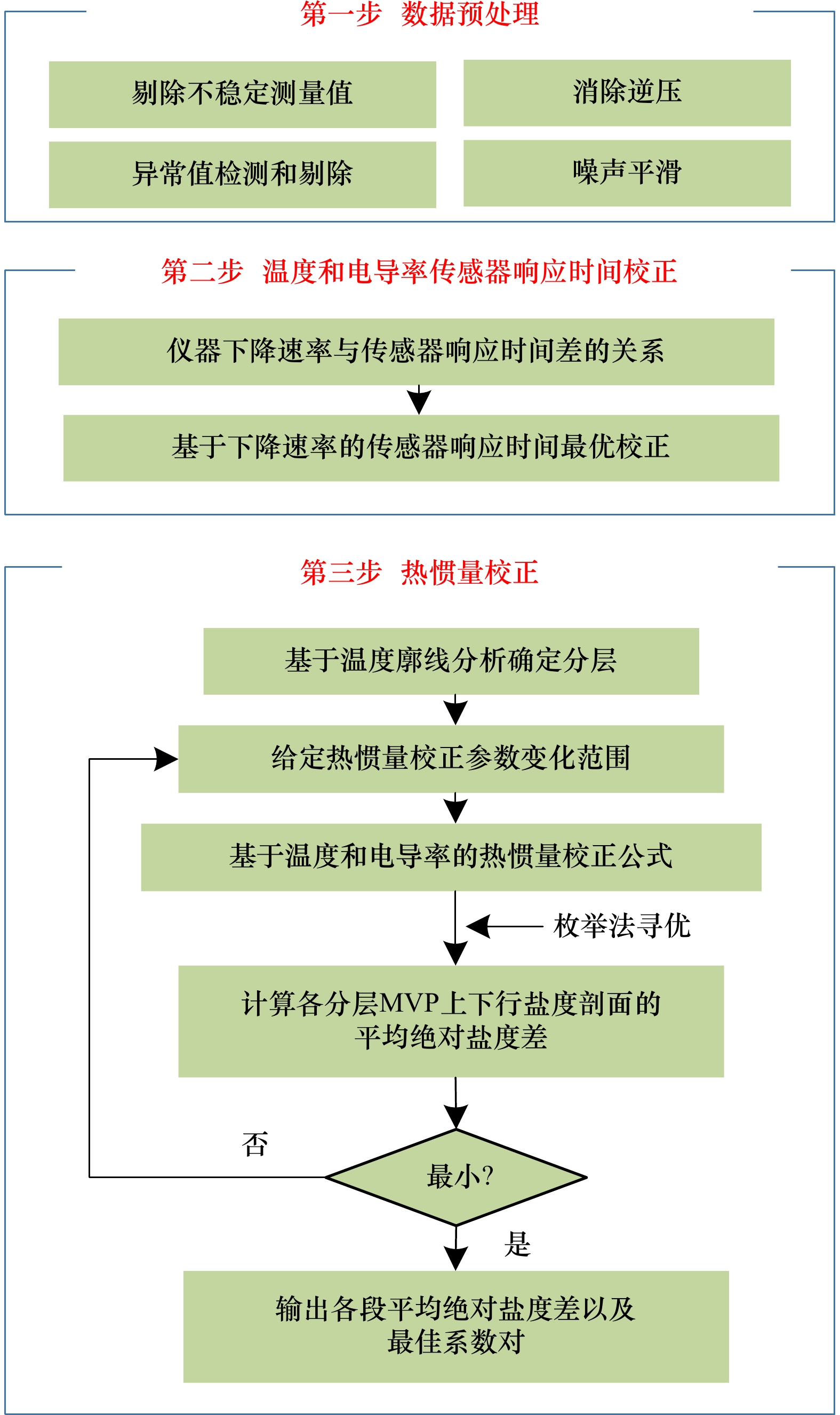
摘要: 走航式海洋剖面测量系统(Moving Vessel Profiler,MVP)具有空间高分辨率温盐剖面探测的优势,但由于采用无泵型CTD进行温盐测量,对测量数据进行传感器响应时间匹配和热惯量校正处理是其数据应用的重点和难点。本文针对现有热惯量校正方法在强温跃层处仍然存在盐度尖峰的局限性,提出一种基于测量温度梯度廓线分析的分层热惯量校正参数寻优方法,校正温度和电导率,进而校正盐度剖面。利用西太平洋某航次实测数据进行试验,结果表明,该方法显著降低了MVP上下行测量剖面的盐度差异,盐度尖峰基本被剔除,特别是温跃层处得到明显改善,上下行剖面的平均绝对盐度差从0.031降低到0.016 1,总体的盐度误差减小48.1%,验证了本文提出的MVP盐度剖面校正方法的合理性。Abstract: The Moving Vessel Profiler (MVP) has the advantage of acquiring temperature and salinity profiles with high spatial resolution. However, since a pumpless CTD is used for the temperature and salinity measurements, adjusting the response time of the sensor and correcting for thermal inertia are important issues in processing the measured data and complicate the application of the data. Since the existing thermal inertia correction methods still have salinity peaks at the strong thermocline, in this work we propose a layered method to optimize the thermal inertia correction parameters based on the analysis of the measured temperature gradient profile to correct the temperature and conductivity, and thus the salinity profile. The results show that the method significantly reduces the salinity difference between the upward and downward measured profiles of the MVP and essentially eliminates the salinity peaks, especially in the thermocline. The average absolute salinity difference between the upward and downward measured profiles is reduced from 0.031 to 0.016 1, which corresponds to a 48.1% reduction in salinity error and confirms the appropriateness of the salinity profile correction method proposed in this work for the MVP.
-

图 4 预处理后307、311和326剖面温度、电导率、盐度和下降速率的深度分布
红线、蓝线和黑线分别代表307、311和326剖面
Fig. 4 Depth distribution of temperature, conductivity, salinity and descent rate of 307, 311 and 326 profiles after pretreatment
The red line, blue line and black line represent 307, 311 and 326 profiles respectively
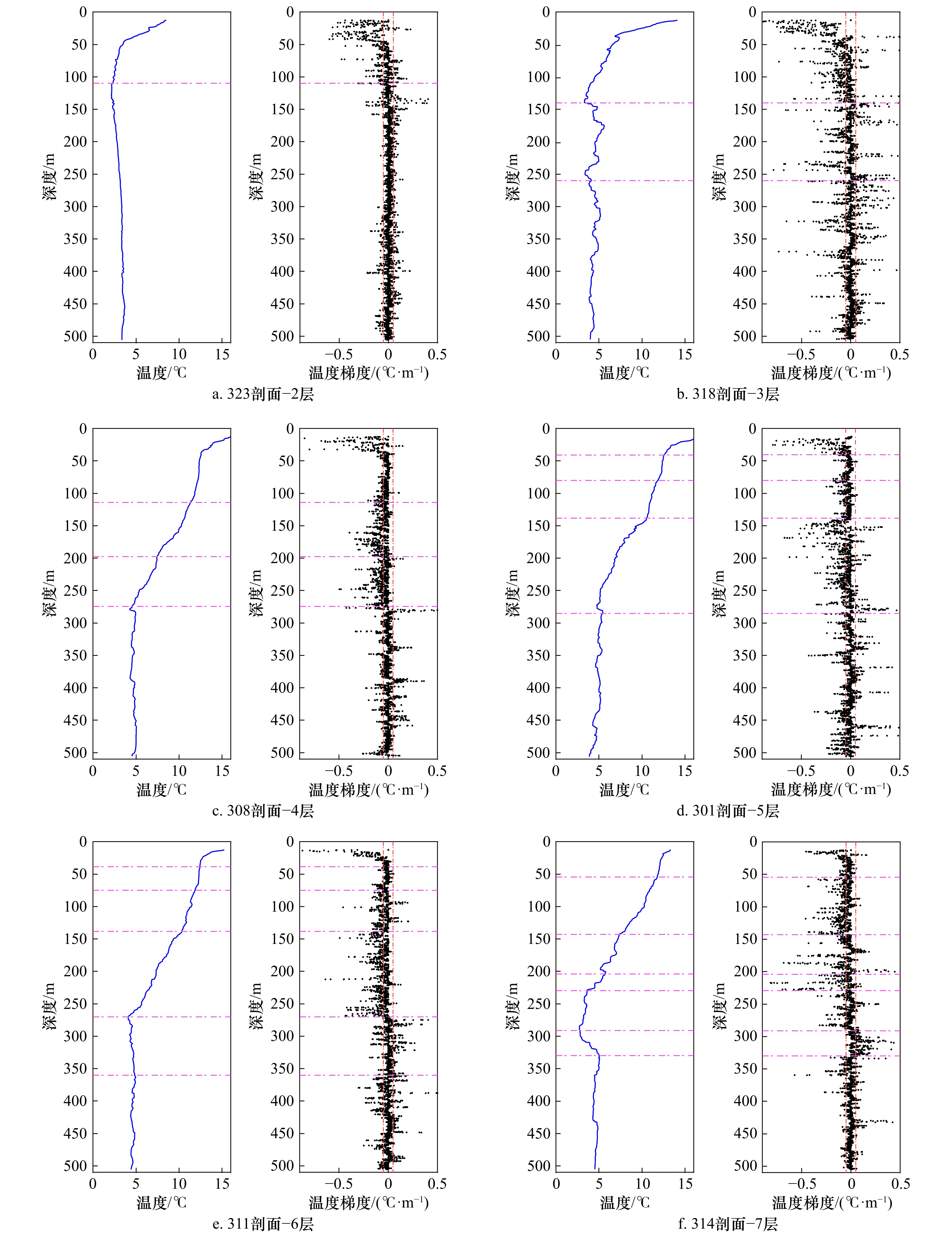
图 5 MVP温度剖面的分层情况
a–f分别是323、318、308、301、311和314剖面的分层情况。每个子图的左图是T–P图,右图是温度梯度随深度的分布图,黑色散点是真实温度梯度散点,红色竖虚线从左至右分别是−0.05 ℃/m和0.05 ℃/m温度梯度阈值线,品红色横虚线是分层界线
Fig. 5 Stratification of MVP temperature profiles
a–f are the stratification of profiles 323, 318, 308, 301, 311 and 314, respectively. The left panel of each subplot is the T–P plot, the right panel is the distribution of temperature gradient with depth, the black scatters are the true temperature gradient scatters, the red dashed lines are the –0.05 ℃/m and 0.05 ℃/m temperature gradient threshold lines from left to right, respectively, and the magenta horizontal dashed line is the stratification boundary

图 6 MVP上下行剖面温度相对电导率的滞后(1点= 0.04 s)随上升/下降速率的变化
Fig. 6 Lag (1 seans = 0.04 s) of relative conductivity of temperature in MVP upstream and downstream profiles with rising/falling rates

图 7 预处理后和传感器响应时间校正后上下行剖面盐度对比
a–c分别为307、311和326剖面的盐度对比图,每个子图的左图为S–P图,红线为传感器响应时间校正后的上下行盐度剖面曲线,蓝线为预处理后的上下行盐度剖面曲线;每个子图的右图为T–S散点图,红点为传感器响应时间校正后的上下行盐度剖面散点,蓝点为预处理后的上下行盐度剖面散点
Fig. 7 Comparison plots of salinity between upstream and downstream profiles after preprocessing and sensor response time correction
a–c Salinity comparison plots for profiles 307, 311, and 326, respectively; the left plot of each subplot is a S–P plot, with the red line showing the up- and down-row salinity profile curves after sensor response time correction, and the blue line showing the up- and down-row salinity profile curves after preprocessing; and the right plot of each subplot is a T–S scatterplot, with the red dots showing the scatters of up- and down-row salinity profiles after sensor response time correction, and the blue dots showing the scatters of up- and down-row salinity profiles after preprocessing
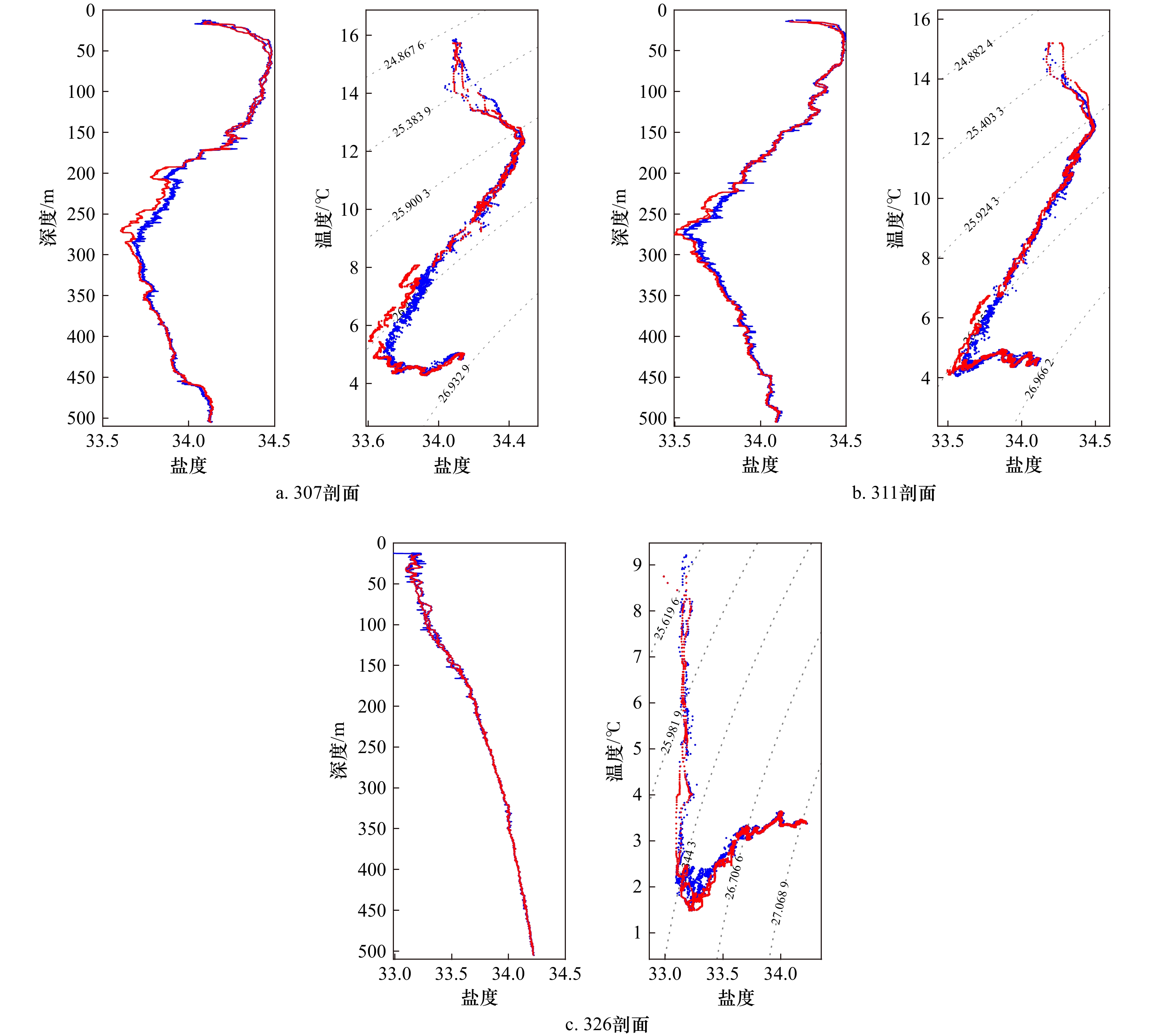
图 8 热惯量订正后与传感器响应时间校正后的上下行剖面的盐度差异
a–c分别为307、311和326剖面的盐度对比图,每个子图的左图为S–P图,红线为热惯量订正后的上下行盐度剖面曲线,蓝线为传感器响应时间校正后的上下行盐度剖面曲线;每个子图的右图为T–S散点图,红点为热惯量订正后的上下行盐度剖面散点,蓝点为传感器响应时间校正后的上下行盐度剖面散点
Fig. 8 Difference in salinity between thermal inertia revised and sensor response time corrected up- and down-row profiles
a–c. Salinity comparison plots for profiles 307, 311, and 326, respectively; the left panel of each subplot is a S–P plot, with the red line showing the upstream and downstream salinity profile curves after thermal inertia revision, and the blue line showing the upstream and downstream salinity profile curves after sensor response time correction; and the right panel of each subplot is a T–S scatter plot, with the red dots showing the upstream and downstream salinity profile scatter points after thermal inertia revision, and the blue dots showing the sensor response time-corrected upstream and downstream salinity profile scatter points in red, and sensor response time-corrected upstream and downstream salinity profile scatter points in blue

图 9 311剖面热惯量校正参数、温度和盐度随深度变化
其中黑线为温度曲线,红线为盐度曲线,绿色、蓝色分段实线为分层热滞后校正最佳系数对,浅绿色、浅蓝色完整线为整层热滞后校正最佳系数对,品红色虚线为分层界线
Fig. 9 The thermal inertia correction parameters, temperature and salinity versus depth for profile 311
The black line is the temperature profile, the red line is the salinity profile, the green and blue segmented solid lines are the best coefficient pairs for the stratified thermal lag correction, the light green and light blue complete lines are the best coefficient pairs for the whole stratified thermal lag correction, and the magenta dashed line is the stratification boundary
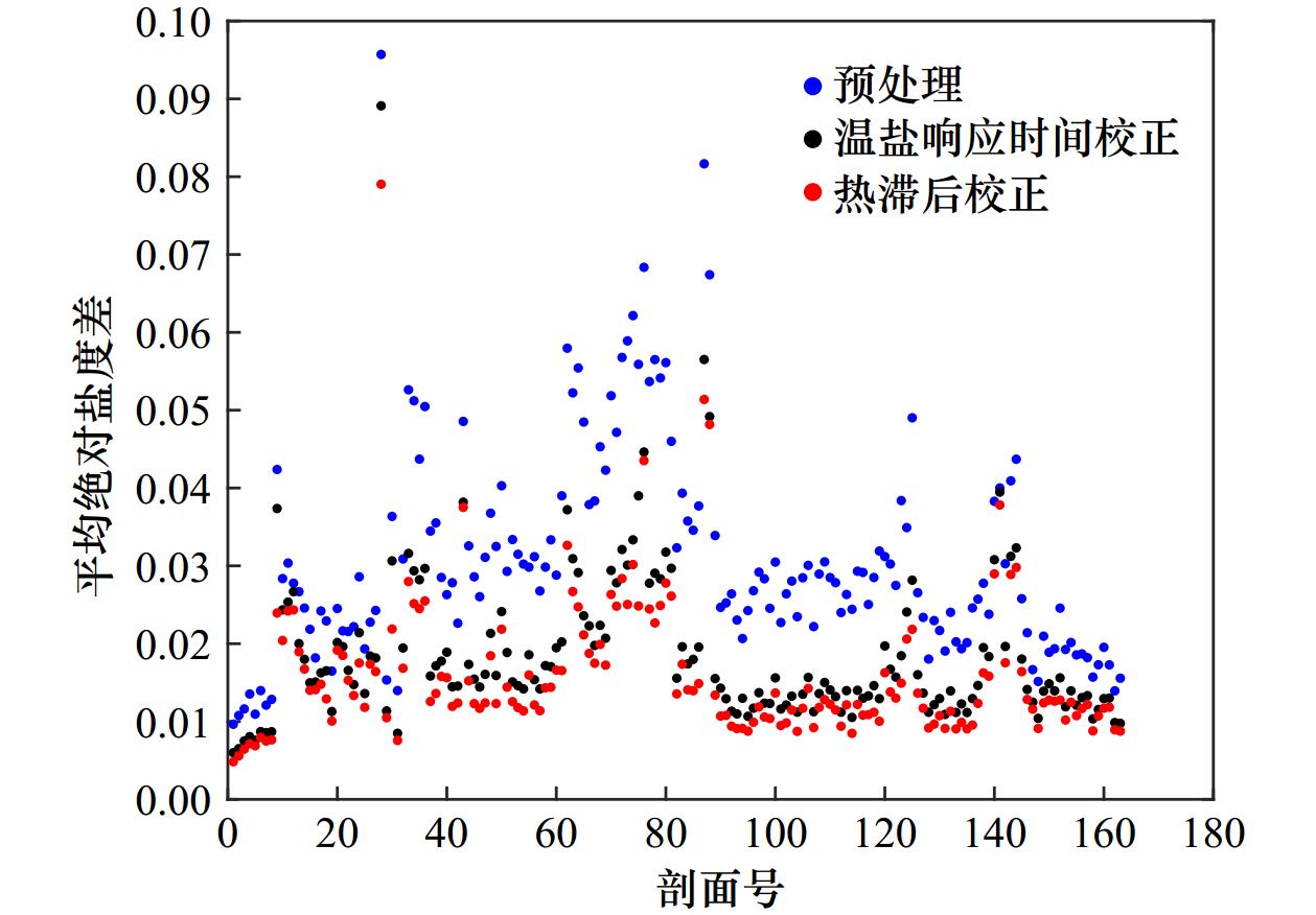
图 10 3步处理过程的平均绝对盐度差
蓝点、黑点和红点分别为预处理过程、传感器响应时间校正和热惯量校正过程的平均绝对盐度差
Fig. 10 Mean absolute salinity difference for the three-step process
The blue, black and red dots are the mean absolute salinity difference for the preprocessing process, sensor response time correction, and thermal inertia correction processes, respectively
表 1 MVP数据剖面分布情况、经纬度及时间范围
Tab. 1 MVP data profile distribution, latitude, longitude and time scale
断面 剖面命名格式 经纬度和时间范围 剖面数 A1 101,102,…,116 2019年5月21–22日
40.67°~41.61°N, 155.53°~155.60°E16 A2 201,202,…,219 2019年5月24日
38.22°~38.91°N, 150.10°~150.49°E19 A3 301,302,…,338 2019年6月6日
40.71°~41.76°N, 145.18°~146.60°E38 A4 401,402,…,498 2019年6月24日
40.96°~42.48°N, 150.29°~150.93°E98  下载: 导出CSV
表 2 预处理后上下行剖面平均绝对盐度差分布情况
Tab. 2 Distribution of mean absolute salinity difference between upstream and downstream profiles after pretreatment
平均绝对盐度差$ |\Delta {S}| $ 剖面号 数目 $ {|\Delta {S}| > 0.031 }$
109、112、207、212、215、216、218、315、316、318、319、402~407、412、413、416~419、421~422、425、
428、430~461、482、492、493、496~49865
$ {0.031\geqslant \left|\Delta {S}\right| > 0.02 }$
110、111、113~116、202、203、205、206、208~210、213、214、301、302、304、305、307、308、310~314、317、
320、321、324、327、329、410、408~411、414~415、420、423、424、426、427、429、462~481、483~491、494、49576
$ {0.02\geqslant \left|\Delta{S}\right| > 0.01} $ 102~108、201、204、211、217、219、303、306、309、322、323、325、326、328、330~338 29 ${ 0.01\geqslant \left|\Delta {S}\right| }$ 101 1
下载: 导出CSV
表 4 温度相对电导率的滞后时间与下降/上升速率的关系
Tab. 4 Temperature relative conductivity lag time versus rate of fall/rise
上行剖面 下行剖面 上升速率/
(m·s-1)温度滞后
电导率/scans下降速率/
(m·s-1)温度滞后
电导率/scans2 –0.183 2.5 1.735 2.25 –0.553 2.75 1.743 2.5 –1.097 3 1.933 2.75 –1.339 3.25 1.942 3 –1.598 3.5 1.922 3.25 –1.925 3.75 2.070 3.5 –2.034 4 2.139 3.75 –2.016 4.25 2.250 4 –1.929 4.5 2.126 4.25 –2.279 4.5 –2.402 4.75 –2.118
下载: 导出CSV
表 5 传感器响应时间校正后上下行剖面平均绝对盐度差分布情况
Tab. 5 Distribution of mean absolute salinity difference between upstream and downstream profiles corrected for sensor response time
平均绝对盐度差$ {|\Delta {S}|} $ 剖面号 数目 $ {\left|\Delta {S}\right| > 0.031} $ 109、112、207、212、215、216、316、318、319、402、412、431、441、443~445、449、453、457~460、482 23 $ {0.031\geqslant \left|\Delta {S}\right| > 0.018\;7} $
110、111、113、114、205、206、210、218、313、315、317、401、403~405、409、417、419、420、
429、430、432~440、442、446~448、450、452、456、493、497~49840
${ 0.018\;7\geqslant \left|\Delta {S}\right| > 0.01} $
115、116、201~204、208、209、211、213、214、217、301~312、314、320~336、406~408、410、
411、413~416、418、421~428、451、454~455、461~481、483~492、494~49697
${ 0.01\geqslant \left|\Delta {S}\right|} $ 101~107、219、337、338 11
下载: 导出CSV
表 6 整层进行热惯量校正后上下行剖面平均绝对盐度差分布情况
Tab. 6 Distribution of mean absolute salinity difference between up and down row profiles after thermal inertia correction for the whole layer
平均绝对盐度差$ {|\Delta {S}| }$ 剖面号 数目 $ {\left|\Delta {S}\right| > 0.031 }$ 112、207、212、215、216、316、412、431、445、453、457~460、482 15 ${ 0.031\geqslant \left|\Delta {S}\right| > 0.018\;7} $
109~111、113、114、205、206、210、218、315、318、319、402~405、419、432~435、437、
439~444、446~450、497、49835
$ {0.018\;7\geqslant \left|\Delta {S}\right| > 0.016\;1} $ 115、213、214、313、314、317、320、401、417、424、429、430、436、438、452、493 16 $ {0.016\;1\geqslant \left|\Delta {S}\right| > 0.01} $
116、201~204、208、209、211、217、301、302、304、305、307、309、311、312、321、322、324~336、
406~411、413~416、418、420~423、425~428、451、454~456、461~463、469~472、475、477、478、
480、481、483、484、486、488~492、494~49679
$ {0.01\geqslant \left|\Delta {S}\right| }$ 101~108、219、303、306、308、310、323、333、337、338、464、465、467、473、474、476、479、485、487 26
下载: 导出CSV
表 7 分段进行热惯量校正后上下行剖面平均绝对盐度差分布情况
Tab. 7 Distribution of the mean absolute salinity difference between upstream and downstream profiles after segmented thermal inertia correction
平均绝对盐度差$ {|\Delta {S}| }$ 剖面号 数目 ${ \left|\Delta {S}\right| > 0.031 }$ 112、207、212、215、216、316、412、431、445、453、457~460、482 15 $ {0.031\geqslant \left|\Delta {S}\right| > 0.018\;7} $ 109~111、113、114、205、218、315、318、319、402~405、419、432~435、437、439~444、446~450、497、498 33 $ {0.018\;7\geqslant \left|\Delta {S}\right| > 0.016\;1 }$ 115、206、210、213、214、313、317、320、401、417、429、430、436、438、452、493 16 $ {0.016\;1\geqslant \left|\Delta {S}\right| > 0.01 }$
116、201~204、208、209、211、217、301、302、305、307、312、314、321、322、324~336、406~411、413~416、418、420~428、451、454~456、461~463、469~472、475、477、478、480、481、483、484、486、488~492、494~496 76
$ {0.01\geqslant \left|\Delta {S}\right|} $ 101~108、219、303、304、306、308~311、323、333、337、338、464~468、473、474、476、479、485、487 31
下载: 导出CSV
表 8 A3断面强温跃层处,分层热惯量校正与整层热惯量校正的效果对比
Tab. 8 Comparison of the effect of stratified thermal inertia correction with that of whole layer thermal inertia correction at the strong thermocline of A3 section
剖面号 强跃层梯度/(℃·m−1) 深度范围/m 平均绝对盐度差 改善效果/% 分层校正 整层校正 301 0.184 12.34~40.73 0.046 2 0.046 3 0.22 302 0.180 12.29~38.74 0.056 1 0.075 9 26.09 303 0.165 12.26~43.93 0.038 7 0.039 1 1.02 304 0.193 12.34~41.16 0.033 4 0.034 4 2.91 306 0.161 12.35~40.11 0.034 7 0.038 9 10.80 307 0.154 12.37~45.95 0.043 8 0.044 2 0.90 308 0.160 12.28~47.33 0.038 8 0.04 0 309 0.177 12.29~39.93 0.046 6 0.047 2 1.27 310 0.181 12.31~45.6 0.013 8 0.013 8 0 311 0.174 12.3~38.32 0.035 0.035 0 316 0.119 16.69~135.47 0.137 6 0.137 6 0 317 0.216 14.4~42.86 0.052 8 0.052 8 0 319 0.267 12.25~49.72 0.266 6 0.266 6 0 321 0.338 12.31~51.84 0.066 2 0.066 6 0.60 322 0.145 12.28~79.83 0.031 6 0.031 6 0 324 0.343 12.33~43.32 0.050 6 0.051 2 1.17 325 0.209 12.28~65.22 0.054 6 0.057 1 4.38 326 0.312 12.34~46.34 0.035 6 0.035 6 0 327 0.269 12.36~54.67 0.061 6 0.079 8 22.81 328 0.273 12.3~62.24 0.022 9 0.022 9 0 329 0.104 12.4~75.53 0.060 8 0.060 9 0.16 330 0.185 12.3~56.41 0.033 9 0.033 9 0 332 0.367 12.28~34.29 0.039 0.039 0 333 0.134 12.26~58.3 0.033 8 0.044 3 23.70 334 0.195 12.26~72.08 0.029 1 0.029 1 0 336 0.175 12.28~74.06 0.044 3 0.044 3 0 337 0.135 12.27~85.13 0.030 6 0.030 6 0 338 0.140 12.33~81.51 0.025 7 0.025 7 0
下载: 导出CSV
-
[1] Fofonoff N P, Hayes S P, Millard R C. W. H. O. I. /Brown CTD microprofiler: methods of calibration and data handling[R]. Woods Hole: Woods Hole Oceanographic Institution, 1974: 1−64. [2] SCOR Working Group 51. The Acquisition, Calibration, and Analysis of CTD Data[M]. Paris: UNESCO Technical Papers in Marine Science, 1988: 94. [3] Giles A B, McDougall T J. Two methods for the reduction of salinity spiking of CTDs[J]. Deep-Sea Research Part A. Oceanographic Research Papers, 1986, 33(9): 1253−1274. doi: 10.1016/0198-0149(86)90023-3 [4] 任强, 于非, 刁新源, 等. 处理走航式海洋多参数剖面测量系统(MVP)温度和电导率滞后效应的方法[J]. 海洋科学, 2014, 38(8): 59−66. doi: 10.11759/hykx20130823002Ren Qiang, Yu Fei, Diao Xinyuan, et al. A data processing method on the hysteresis effect of temperature and conductivity of moving vessel profiler (MVP)[J]. Marine Sciences, 2014, 38(8): 59−66. doi: 10.11759/hykx20130823002 [5] Ullman D S, Hebert D. Processing of underway CTD data[J]. Journal of Atmospheric and Oceanic Technology, 2014, 31(4): 984−998. doi: 10.1175/JTECH-D-13-00200.1 [6] Barth J A, O’Malley R, Fleischbein J, et al. SeaSoar and CTD observations during the Coastal Jet Separation cruise W9408A, August to September 1994[R]. College of Oceanic and Atmospheric Sciences, Oregon State University, 1996: 170. [7] Lueck R G. Thermal inertia of conductivity cells: theory[J]. Journal of Atmospheric and Oceanic Technology, 1990, 7(5): 741−755. doi: 10.1175/1520-0426(1990)007<0741:TIOCCT>2.0.CO;2 [8] Lueck R G, Picklo J J. Thermal inertia of conductivity cells: observations with a sea-bird cell[J]. Journal of Atmospheric and Oceanic Technology, 1990, 7(5): 756−768. doi: 10.1175/1520-0426(1990)007<0756:TIOCCO>2.0.CO;2 [9] Morison J, Andersen R, Larson N, et al. The correction for thermal-lag effects in sea-bird CTD data[J]. Journal of Atmospheric and Oceanic Technology, 1994, 11(4): 1151−1164. doi: 10.1175/1520-0426(1994)011<1151:TCFTLE>2.0.CO;2 [10] Mensah V, Le Menn M, Morel Y. Thermal mass correction for the evaluation of salinity[J]. Journal of Atmospheric and Oceanic Technology, 2009, 26(3): 665−672. doi: 10.1175/2008JTECHO612.1 [11] Garau B, Ruiz S, Zhang W G, et al. Thermal lag correction on Slocum CTD glider data[J]. Journal of Atmospheric and Oceanic Technology, 2011, 28(9): 1065−1071. doi: 10.1175/JTECH-D-10-05030.1 [12] Liu Zenghong, Xu Jianping, Yu Jiancheng. Real-time quality control of data from Sea-Wing underwater glider installed with Glider Payload CTD sensor[J]. Acta Oceanologica Sinica, 2020, 39(3): 130−140. doi: 10.1007/s13131-020-1564-6 [13] U. S. Integrated Ocean Observing System. Manual for quality control of temperature and salinity data observations from gliders Version 1.0[EB/OL]. (2011−12-01) [2018−08−16]. https://cdn.ioos.noaa.gov/media/2017/12/Manual-for-QC-of-Glider-Data_05_09_16.pdf. [14] Liu Yonggang, Weisberg R H, Lembke C. Chapter 17-Glider salinity correction for Unpumped CTD sensors across a sharp thermocline[M]//Liu Yonggang, Kerkering H, Weisberg R H. Coastal Ocean Observing Systems. Amsterdam: Academic Press, 2015: 305−325. [15] 张学宏, 张绪东, 李颜. 海洋温跃层特征值的分析与计算[J]. 海洋预报, 2011, 28(5): 69−76. doi: 10.3969/j.issn.1003-0239.2011.05.011Zhang Xuehong, Zhang Xudong, Li Yan. Characteristic analysis and calculation of the ocean thermocline[J]. Marine Forecasts, 2011, 28(5): 69−76. doi: 10.3969/j.issn.1003-0239.2011.05.011 -


计量
- 文章访问数: 335
- HTML全文浏览量: 209
- PDF下载量: 29
- 被引次数: 0
