

Temperature profile inversion in the South China Sea under the constraint of depth-fixed temperature
-
摘要: 为快速获取大范围、准实时的海洋内部结构,海面遥感数据被广泛应用于构建温度剖面垂直结构,但卫星遥感仅能获得较为准确的海洋表面或者近表层数据。为了提高全海深温度剖面的反演精度,本文以水下固定深度处温度为约束,通过径向基函数神经网络生成海表面温度和海平面高度异常等海表遥感数据与温度剖面之间的非线性映射,并对约束深度选取的理论依据进行讨论。南海海域温度剖面的反演结果表明,第1阶经验正交函数系数可以表征温跃层的垂直位移,而第1阶经验正交函数基函数极值点对应深度处的温度与第1阶经验正交函数系数之间具有强相关性。当增加该深度处温度为约束时,温跃层的反演精度比仅使用海面遥感数据约提高0.35℃,反演温度剖面的平均均方根误差约为0.33℃。Abstract: In order to quickly obtain a large-scale, quasi-real-time internal structure of the ocean, sea surface remote sensing data are widely used to construct the vertical structure of the temperature profiles, but satellite remote sensing can only obtain relatively accurate ocean surface or near-surface data. In order to improve the accuracy of temperature profile inversion, this paper takes the depth-fixed temperature as the constraint, and the nonlinear mapping between the temperature profiles and the sea surface remote sensing data such as sea surface temperature (SST) and sea level anomaly (SLA) is generated through the radial basis function (RBF) neural network, and discuss the theoretical basis for constrained depth selection. The inversion results of the temperature profiles in the South China Sea show that the first empirical orthogonal function (EOF) coefficient can characterize the vertical displacement of the thermocline. And there is a strong correlation between the temperature at the depth corresponding to the extreme point of the first EOF and the first EOF coefficient. Therefore, when the temperature at this depth is added as a constraint, the inversion accuracy of the thermocline is about 0.35℃ higher than that of only using sea surface remote sensing data, and the mean root mean square error of temperature profile inversion is about 0.33℃.
-
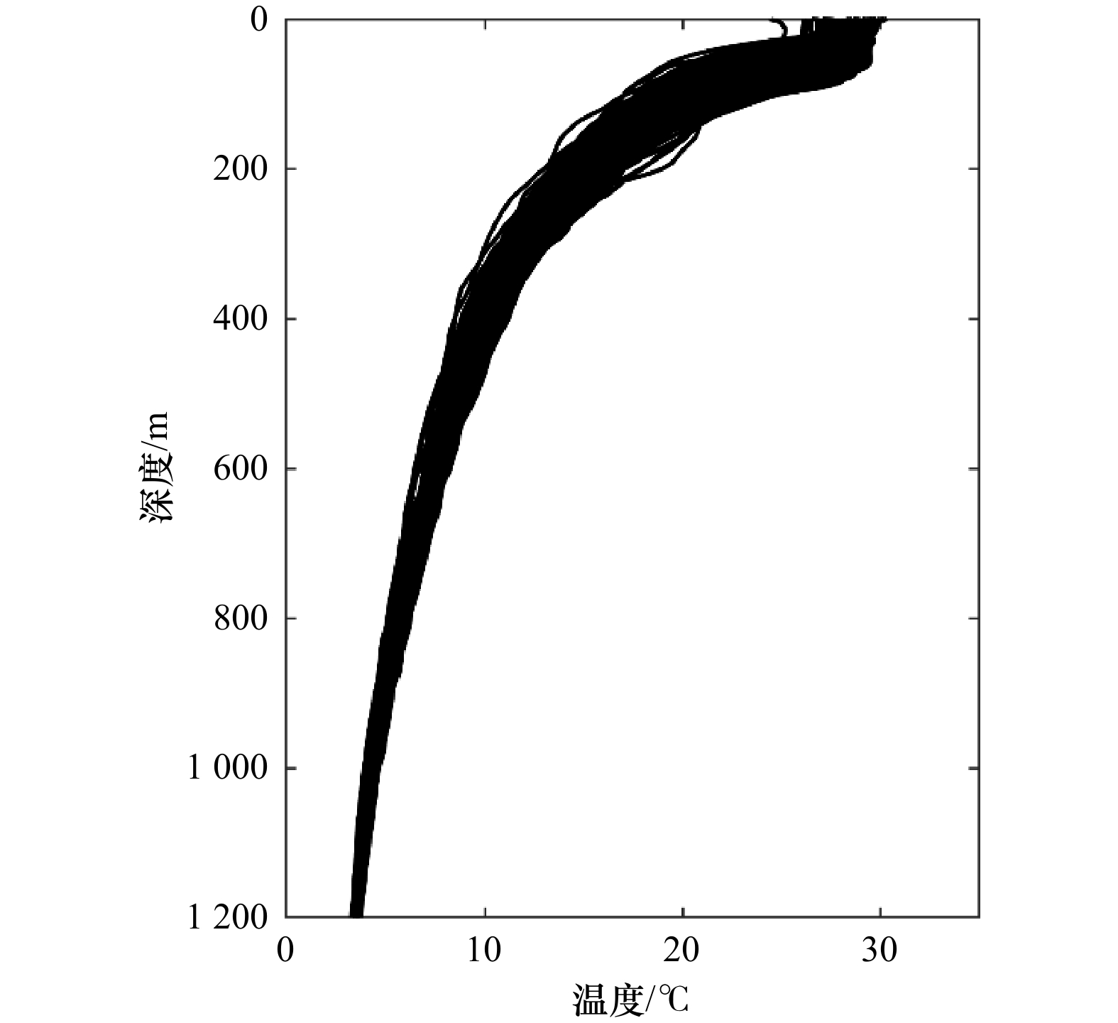
图 2 1 200 m以浅的温度剖面
Fig. 2 Measure temperature profiles at depths shallower than 1 200 m
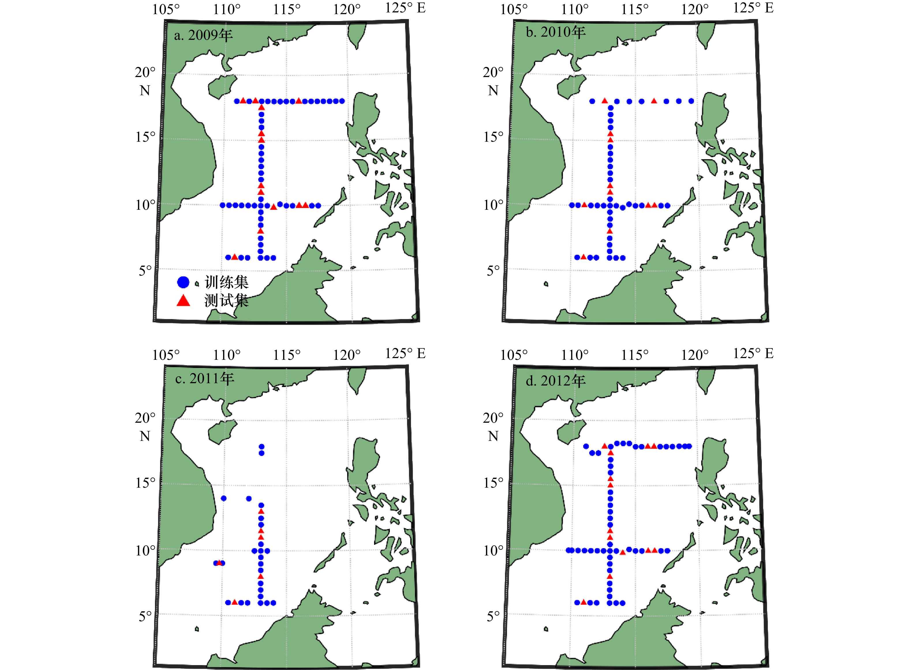
图 3 训练集与测试集站位的空间分布
Fig. 3 Spatial distribution of stations in the training and test sets
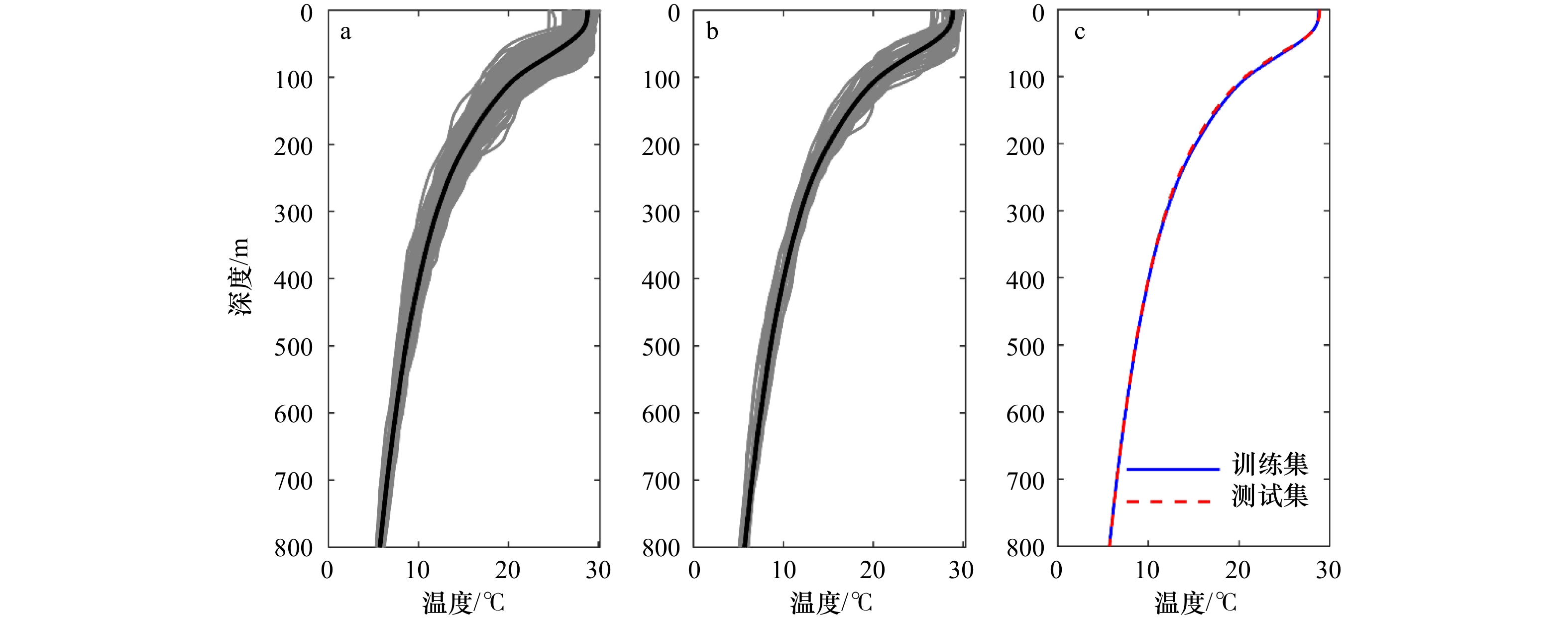
图 4 训练集(a)、测试集(b)温度剖面及训练集和测试集平均温度剖面(c)
灰色实线为实测温度剖面,黑色实线为平均温度剖面
Fig. 4 Temperature profiles in the training set (a) and test set (b), and mean temperature profiles of training and test sets (c)
The gray solid line represents the measured temperature profile, while the black solid line represents the average temperature profile
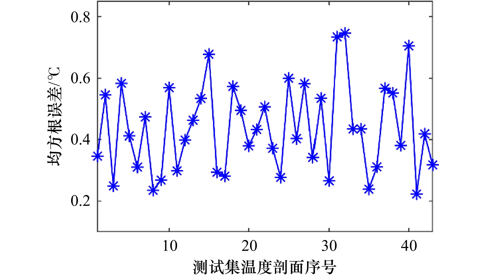
图 6 位置信息和遥感数据反演温度剖面的均方根误差
Fig. 6 Root mean square error of temperature profile inversion using position information and remote sensing data

图 7 不同约束温度下的温度剖面重构误差与第1阶EOF基函数的对比(归一化后)
Fig. 7 Comparison of the temperature profile reconstruction error at different confinement temperatures and the first EOF (after normalization)
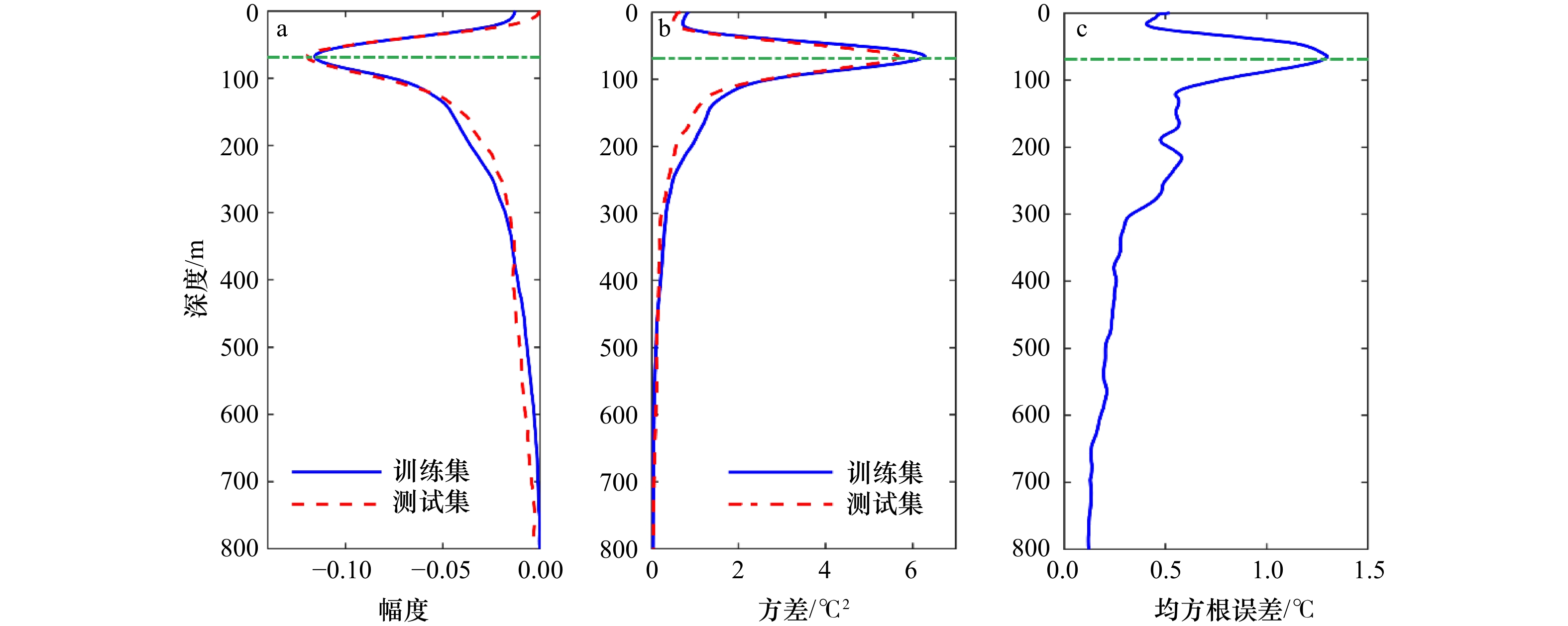
图 8 训练集和测试集第1阶EOF基函数(a),温度剖面的方差(b)及 均方根误差随深度的变化(c)
Fig. 8 The first EOF (a) , variance of the temperature profiles (b) and root mean square error with depth (c) of training set and test set
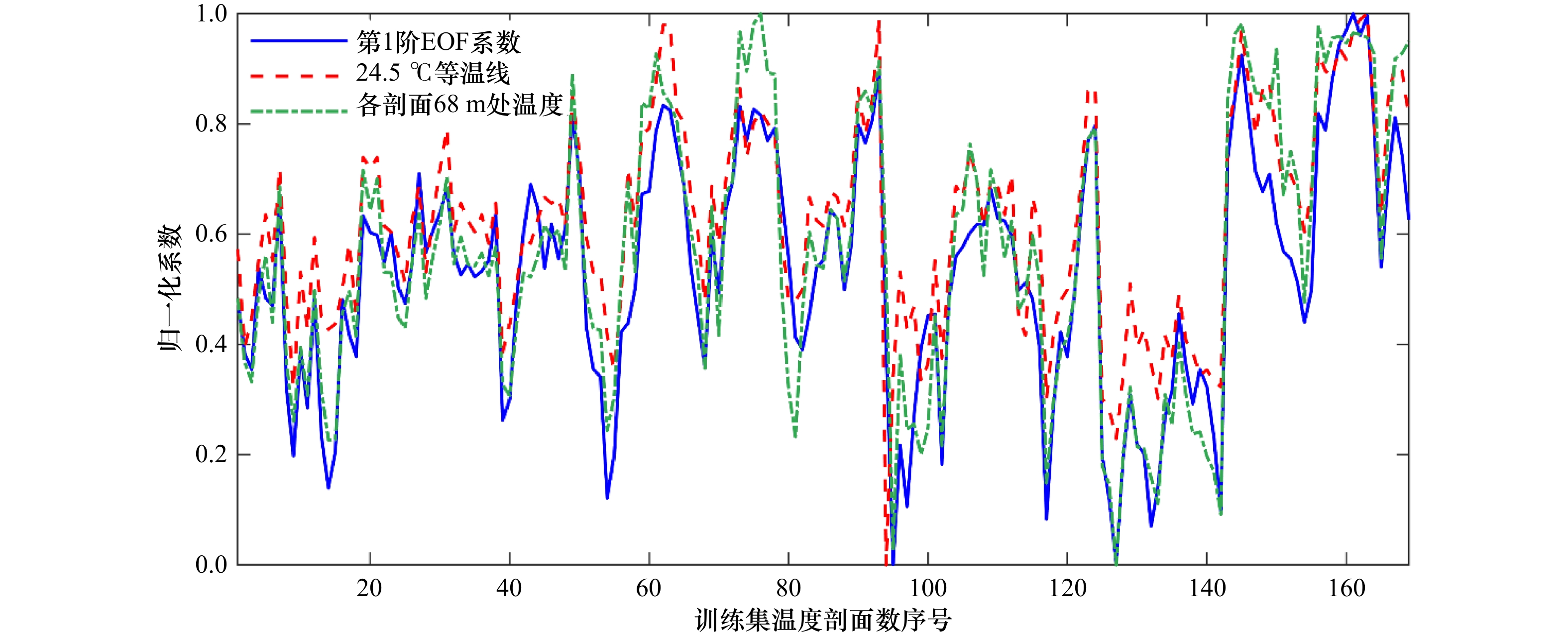
图 9 第1阶EOF系数、24.5℃等温线及各剖面68 m处温度(归一化后)
Fig. 9 The first EOF coefficient, 24.5°C isotherm and temperature at 68 m of each profile (after normalization)
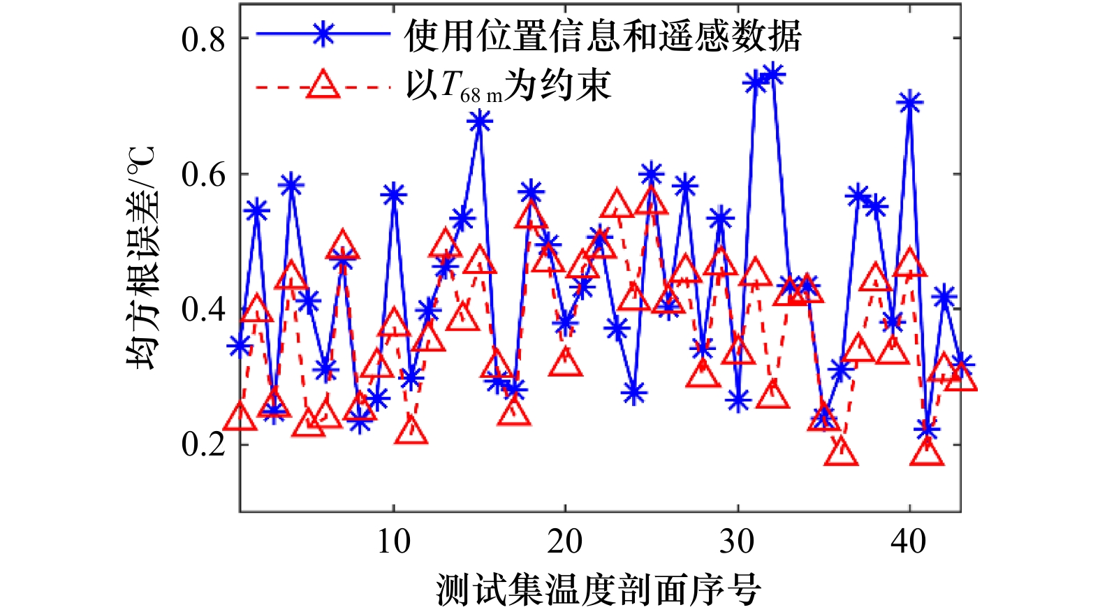
图 10 使用两种方法反演温度剖面的均方根误差
Fig. 10 Root mean square error of the temperature profile inversion using two methods
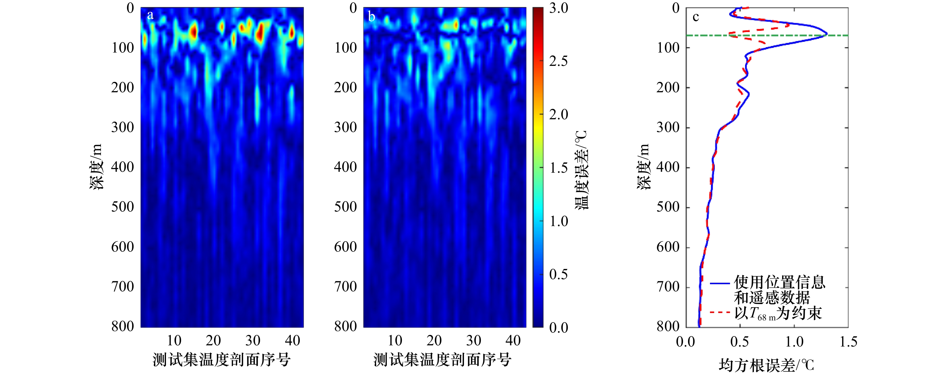
图 11 温度剖面反演误差随深度的分布
a. 使用位置信息和遥感数据;b. 以T68 m为约束;c. 均方根误差随深度的变化
Fig. 11 Distribution of temperature profile inversion error with depth
a. Using position information and remote sensing data; b. constrained by T68 m; c. root mean square error with depth
表 1 前6阶EOF方差贡献率及累计方差贡献率
Tab. 1 First six EOFs variance contribution and cumulative variance contribution
EOF阶次 训练集 测试集 方差贡献率/
%累计方差贡献率/
%方差贡献率/
%累计方差贡献率/
%1 68.99 68.99 69.15 69.15 2 12.02 81.01 11.82 80.97 3 7.24 88.25 7.81 88.78 4 4.05 92.30 3.96 92.74 5 2.64 94.94 2.55 95.29 6 1.55 96.49 1.91 97.20  下载: 导出CSV
表 2 深度浮动对反演温度剖面的均方根误差(RMSE)影响
Tab. 2 Influence of depth fluctuation on root mean square error (RMSE) of temperature profile inversion
实验a RMSEn RMSEm 最大值 平均值 最大值 平均值 未考虑深度浮动 0.555 3 0.367 4 0.948 3 0.3307 1 0.555 8 0.365 9 0.946 2 0.330 1 2 0.556 2 0.367 1 0.947 6 0.330 5 3 0.556 1 0.367 8 0.954 1 0.330 9 4 0.557 6 0.366 8 0.953 5 0.330 5
下载: 导出CSV
表 3 温度测量误差对反演温度剖面的均方根误差(RMSE)影响
Tab. 3 Influence of temperature measurement error on root mean square error (RMSE) of temperature profile inversion
实验b RMSEn RMSEm 最大值 平均值 最大值 平均值 1 0.573 7 0.364 7 0.959 5 0.329 0 2 0.557 7 0.366 3 0.949 7 0.330 1 3 0.555 8 0.367 5 0.948 3 0.330 8 4 0.554 9 0.366 9 0.947 0 0.330 3
下载: 导出CSV
表 4 深度浮动和温度测量误差对反演温度剖面的均方根误差(RMSE)影响
Tab. 4 Influence of depth fluctuation and temperature measurement error on root mean square error (RMSE) of temperature profile inversion
实验c RMSEn RMSEm 最大值 平均值 最大值 平均值 1 0.575 4 0.369 3 0.949 2 0.333 9 2 0.556 7 0.366 8 0.951 1 0.330 3 3 0.555 2 0.370 0 0.941 9 0.333 9 4 0.556 2 0.366 9 0.952 1 0.330 5
下载: 导出CSV
-
[1] 修树孟, 张钦, 逄爱梅. 卫星遥感SST反演海水温度垂直剖面的方法研究[J]. 遥感信息, 2009(5): 73−76.Xiu Shumeng, Zhang Qin, Pang Aimei. Asimulation of the seawater temperature vertical profile from satellite SST observation[J]. Remote Sensing Information, 2009(5): 73−76. [2] Li Haipeng, Qu Ke, Zhou Jianbo. Reconstructing sound speed profile from remote sensing data: nonlinear inversion based on self-organizing map[J]. IEEE Access, 2021, 9: 109754−109762. [3] Guinehut S, Le Traon P Y, Larnicol G, et al. Combining Argo and remote-sensing data to estimate the ocean three-dimensional temperature fields—A first approach based on simulated observations[J]. Journal of Marine Systems, 2004, 46(1/4): 85−98. [4] Fujii Y, Kamachi M. Three-dimensional analysis of temperature and salinity in the equatorial Pacific using a variational method with vertical coupled temperature-salinity empirical orthogonal function modes[J]. Journal of Geophysical Research: Oceans, 2003, 108(C9): 3297. doi: 10.1029/2002JC001745 [5] 邢霄波, 徐永生, 贾永君, 等. 基于遥感数据的三维温度场参数化分析方法研究[J]. 海洋学报, 2020, 42(11): 39−48.Xing Xiaobo, Xu Yongsheng, Jia Yongjun, et al. Research on parameterized analysis method of 3D temperature field based on remote sensing data[J]. Haiyang Xuebao, 2020, 42(11): 39−48. [6] Lapeyre G, Klein P. Dynamics of the upper oceanic layers in terms of surface quasigeostrophy theory[J]. Journal of Physical Oceanography, 2006, 36(2): 165−176. doi: 10.1175/JPO2840.1 [7] Lu Wenfang, Su Hua, Yang Xin, et al. Subsurface temperature estimation from remote sensing data using a clustering-neural network method[J]. Remote Sensing of Environment, 2019, 229: 213−222. doi: 10.1016/j.rse.2019.04.009 [8] Munk W, Wunsch C. Ocean acoustic tomography: a scheme for large scale monitoring[J]. Deep-Sea Research Part A. Oceanographic Research Papers, 1979, 26(2): 123−161. doi: 10.1016/0198-0149(79)90073-6 [9] Sagen H, Dushaw B D, Skarsoulis E K, et al. Time series of temperature in Fram Strait determined from the 2008–2009 DAMOCLES acoustic tomography measurements and an ocean model[J]. Journal of Geophysical Research: Oceans, 2016, 121(7): 4601−4617. doi: 10.1002/2015JC011591 [10] 廖光洪, 朱小华, 林巨, 等. 海洋声层析观测技术和方法[J]. 海洋学报, 2010, 32(3): 14−22.Liao Guanghong, Zhu Xiaohua, Lin Ju, et al. Observation technology and methods of ocean acoustic tomography[J]. Haiyang Xuebao, 2010, 32(3): 14−22. [11] Melo J, Matos A. Guidance and control of an ASV in AUV tracking operations[C]//OCEANS 2008. Quebec City, QC, Canada: IEEE, 2008: 1−7. [12] Liu Chuan, Xiang Xianbo, Yang Lichun, et al. A hierarchical disturbance rejection depth tracking control of underactuated AUV with experimental verification[J]. Ocean Engineering, 2022, 264: 112458. doi: 10.1016/j.oceaneng.2022.112458 [13] Xu Hao, Zhang Guocheng, Sun Yushan, et al. Design and experiment of a plateau data-gathering AUV[J]. Journal of Marine Science and Engineering, 2019, 7(10): 376. doi: 10.3390/jmse7100376 [14] 孙春健, 张晓爽, 张寅权, 等. 卫星遥感重构海洋次表层研究进展[J]. 海洋信息, 2018, 33(4): 21−28. doi: 10.19661/j.cnki.mi.2018.04.004Sun Chunjian, Zhang Xiaoshuang, Zhang Yinquan, et al. Progress in reconstruction of ocean subsurface by satellite remote sensing data[J]. Marine Information, 2018, 33(4): 21−28. doi: 10.19661/j.cnki.mi.2018.04.004 [15] Yu Siyuan, Wu Wenhua, Xie Bin, et al. Extreme value prediction of current profiles in the South China Sea based on EOFs and the ACER method[J]. Applied Ocean Research, 2020, 105: 102408. doi: 10.1016/j.apor.2020.102408 [16] Moody J, Darken C J. Fast learning in networks of locally-tuned processing units[J]. Neural Computation, 1989, 1(2): 281−294. doi: 10.1162/neco.1989.1.2.281 [17] Reynolds R W, Smith T M, Liu Chunying, et al. Daily high-resolution-blended analyses for sea surface temperature[J]. Journal of Climate, 2007, 20(22): 5473−5496. doi: 10.1175/2007JCLI1824.1 [18] AVISO. SSALTO/DUACS User Handbook: (M)SLA and (M)ADT Near-real Time and Delayed Time Products[M]. Paris: CNES, 2012. [19] 徐超, 李莎, 陈荣裕, 等. 2009−2012年南海海洋断面科学考察CTD温盐观测数据集[J]. 中国科学数据, 2016(3): 13−18.Xu Chao, Li Sha, Chen Rongyu, et al. CTD observation dataset of scientific investigation over the South China Sea (2009−2012)[J]. China Scientific Data, 2016(3): 13−18. [20] 钟玮琪, 屈科, 梁羿. 基于经验正交函数的剖面重构及其物理意义分析[J]. 海洋技术学报, 2022, 41(1): 57−64. doi: 10.3969/j.issn.1003-2029.2022.01.008Zhong Weiqi, Qu Ke, Liang Yi. Profile reconstruction based on empirical orthogonal function and its physical meaning analysis[J]. Ocean Technology, 2022, 41(1): 57−64. doi: 10.3969/j.issn.1003-2029.2022.01.008 -


计量
- 文章访问数: 586
- HTML全文浏览量: 227
- PDF下载量: 44
- 被引次数: 0
