

Calculation of extreme water level with the effect of sea level rise
-
摘要: 本研究基于非平稳序列极值理论,定量分析极端水位事件年超越概率受海平面上升的影响;以工程设计使用年限内极端水位发生概率作为控制条件,构建考虑海平面上升的极值水位计算方法;结合平均海平面的长期变化过程,推算海平面上升下的极值水位。基于全球10个验潮站历史水位观测资料,验证历史平均海平面长期变化与高、低水位耿贝尔分布位置参数变化的一致性以及构建方法的合理性。结合政府间气候变化专门委员会对海平面上升的预测,推算和对比分析不同海平面上升情景下的极值水位,并评估相应极值水位在当前极值分布中的重现期。Abstract: Based on the extreme value theory of non-stationary sequences, this study carried out the quantitative analysis of the effect of sea level rise on the exceedance probability of extreme water levels. A new method for the estimation of extreme water level with sea level rise was proposed by adopting the overall exceedance probability of extreme water level within the design lifetime of coastal facilities as a critical constraint. With the incorporation of sea level rise in the location parameter of Gumbel distribution, the new method allows the adjustment of the annual exceedance probability of extreme water levels along with sea level rise over time. The validity of the proposed method was examined using the long term sea level measurement data at 10 tide gauge stations globally. Using the five global mean sea level rise scenarios projected by IPCC, the extreme water levels for different design lifetime of coastal facilities with sea level rise were estimated, and the return periods of the extreme water levels were also evaluated.
-
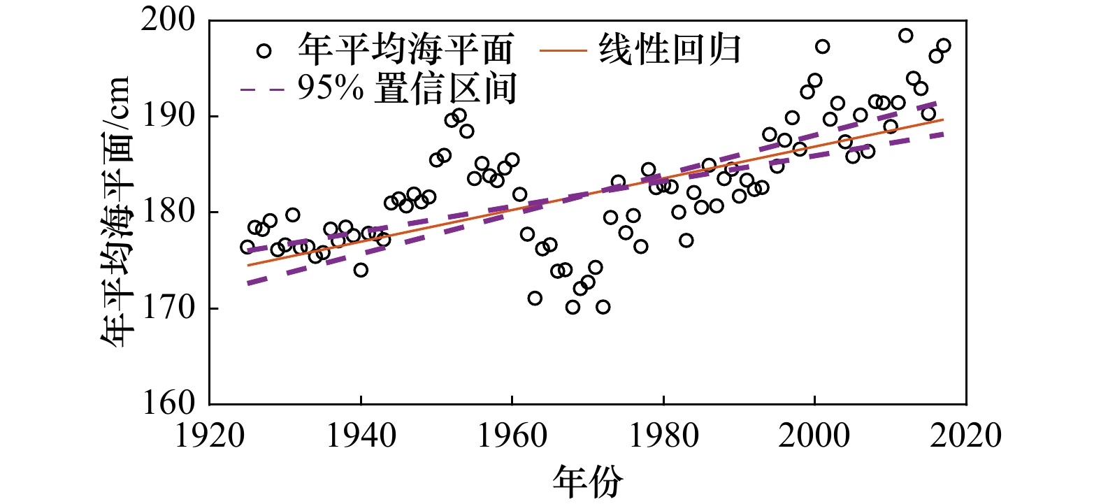
图 1 澳门验潮站1925–2017年平均海平面及其线性趋势
Fig. 1 Annual mean sea level and its linear regression for Macao tide gauge station between the year 1925 and 2017
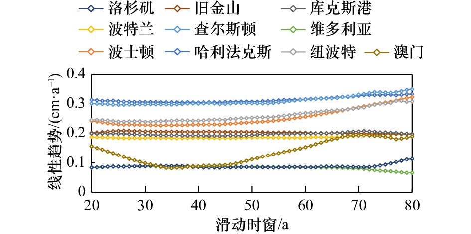
图 2 20~80年滑动时窗下各验潮站平均海平面的线性趋势
Fig. 2 Linear trends of mean sea levels with running time window ranging from 20 a to 80 a at the 10 tide gauge stations

图 3 20~80 a滑动时窗下各验潮站处平均海平面线性趋势的相对误差
Fig. 3 Relative errors of the linear trends of mean sea levels with running time window ranging from 20 a to 80 a at the 10 tide gauge stations
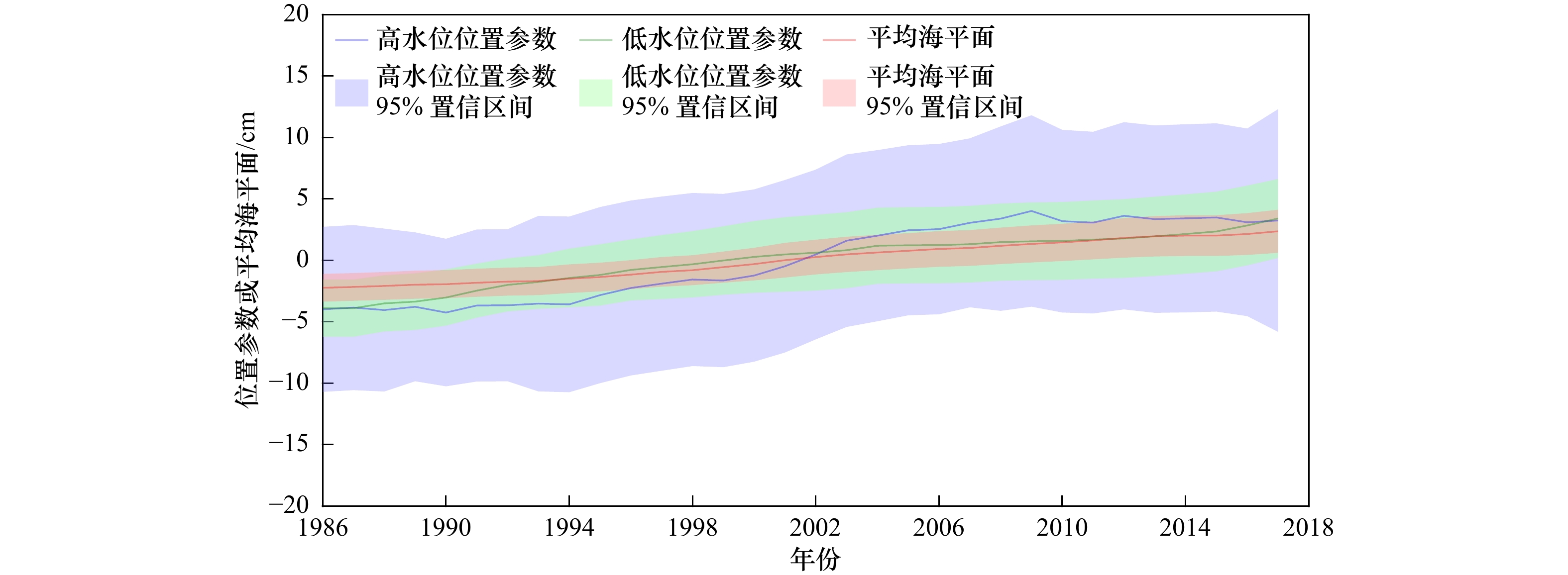
图 4 62 a滑动时窗下澳门验潮站平均海平面和高、低水位耿贝尔分布位置参数历时曲线
图中平均海平面和高、低水位耿贝尔分布位置参数均为减去相应历时范围内平均值的结果
Fig. 4 Time series of mean sea level and location parameters of Gumbel distribution with the 62 a running time window at Macao tide gauge station
The mean sea level and location parameters of Gumbel distribution are results subtracted by the corresponding time averaged values
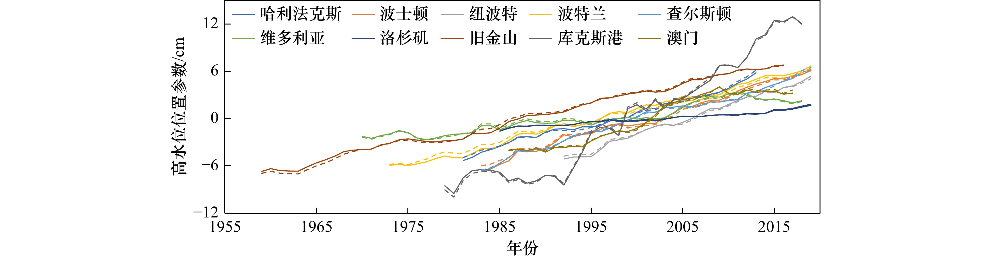
图 5 62 a滑动时窗下各验潮站高水位位置参数(实线)与去除年平均海平面的高水位位置参数和相应平均海平面线性叠加(虚线)的比较
图中各高水位位置参数为减去相应历时范围内平均值的结果
Fig. 5 Comparison between location parameters of the Gumbel distribution for the annual high water levels (solid lines) and the linear summation of mean sea level and location parameters of the Gumbel distribution for the annual high water levels subtracted by annual mean sea level (dash lines)
The location parameters of Gumbel distribution are results subtracted by the corresponding time-averaged values

图 6 澳门验潮站平均海平面与高、低水位耿贝尔分布位置参数的线性回归
Fig. 6 Linear regressions of location parameters of the Gumbel distribution for the annual high and low water levels using the long term mean sea level at Macao tide gauge station
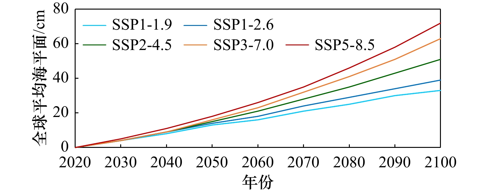
图 7 不同温室气体排放情景下全球海平面相对于2020年的上升预测
根据IPCC第6次评估报告[1]中图SPM.8(d)修改,仅给出各温室气体排放情景下海平面上升预测中值
Fig. 7 Prediction of the global mean sea level rise relative to the year of 2020 under different greenhouse gas emission scenarios
The plot is adapted from Figure SMP.8(d) in the IPCC AR6[1] and only the medium values of the prediction results for different greenhouse gas emission scenarios were given
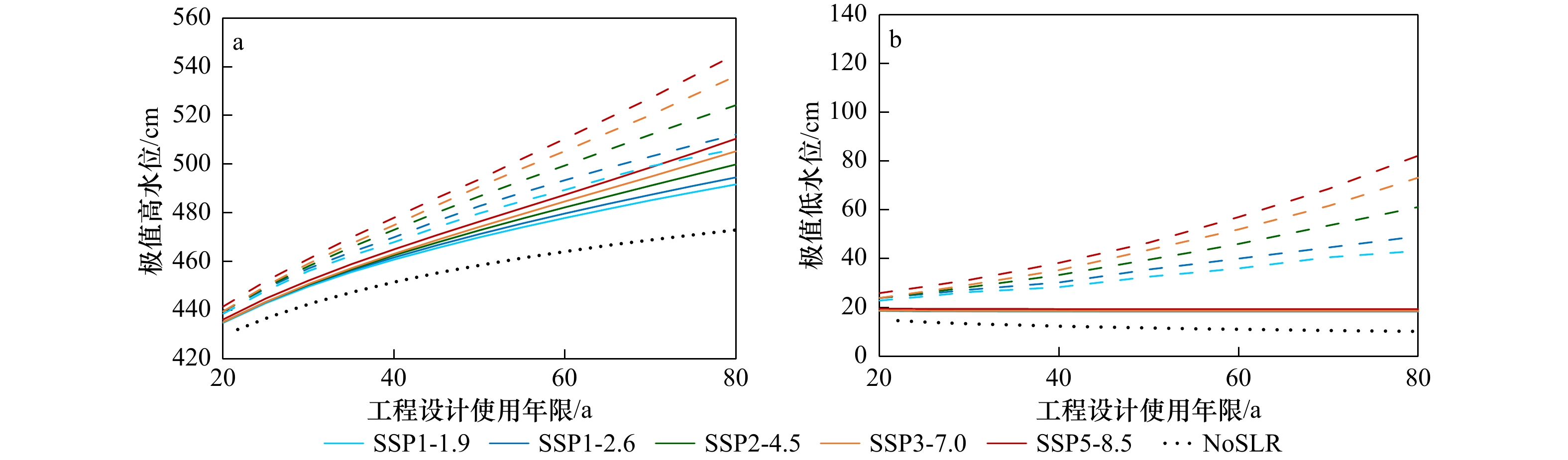
图 8 不同温室气体排放情景下澳门验潮站处各工程设计使用年限极值高、低水位比较
实线为采用本文构建方法计算的考虑海平面上升的极值水位(结合IPCC第6次评估报告中对海平面上升的预测),虚线以当前极值水位线性叠加工程设计使用年限内IPCC对海平面上升的预测值作为极值水位,黑色圆点线(NoSLR)为不考虑海平面上升的极值水位
Fig. 8 Comparion of extreme high and low water levels for different design lifetime under different greenhouse gas emission scenarios at Macao tide gauge station
The solid lines represent results using the method constructed in this paper; the dash lines represent results by adding the predicted mean sea level rise within the design lifetime to the current extreme water level without considering sea-level rise; the black dotted lines represent results without considering sea level rise
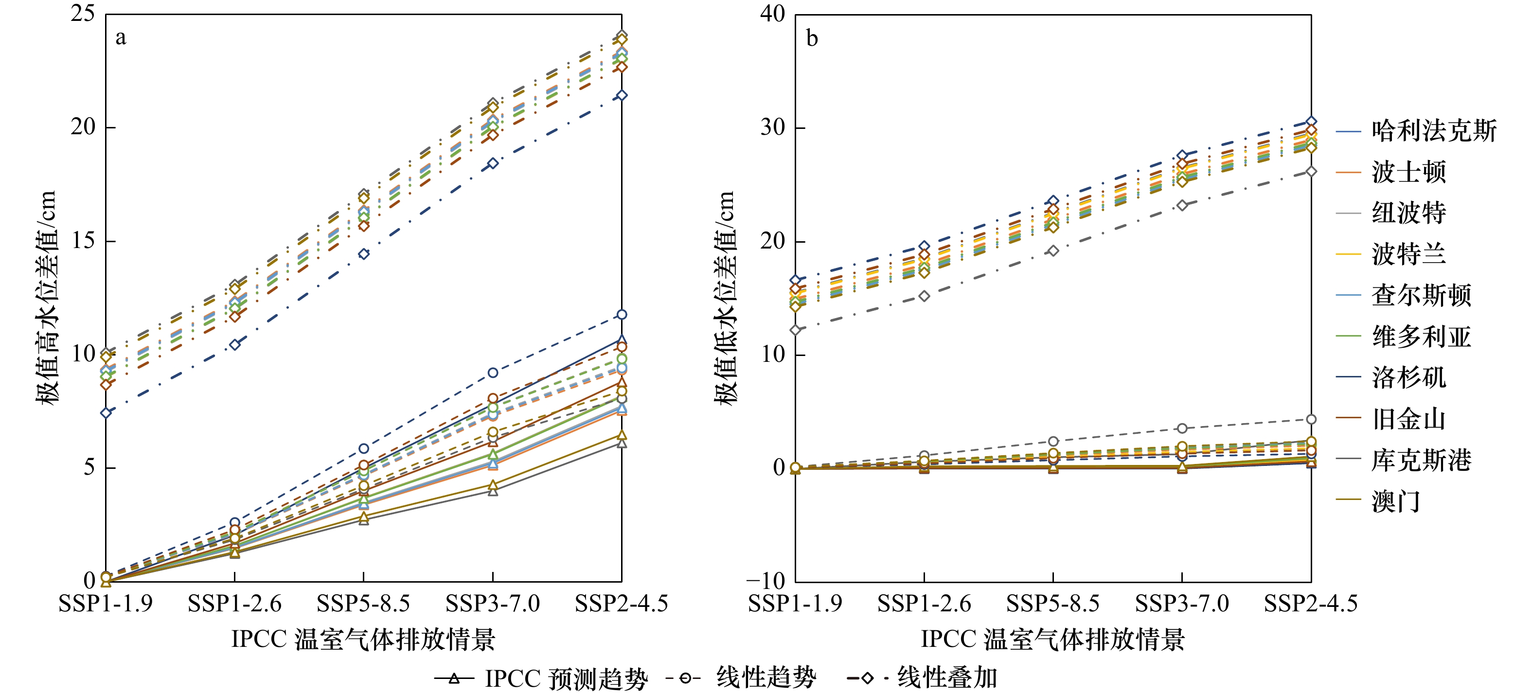
图 9 工程设计使用年限为50 a时不同温室气体排放情景下各验潮站极值高、低水位比较
图中极值高/低水位差值为各验潮站极值高/低水位减去相应验潮站处温室气体极低排放情景(SSP1-1.9)下本文构建方法计算的“IPCC预测趋势”下极值高/低水位的值
Fig. 9 Comparison of extreme high and low water levels for the design lifetime of 50 a under different greenhouse gas emission scenarios
The difference of extreme high/low water levels are the extreme high/low water levels subtracted by the results calculated by the method constructed in this paper under the greenhouse gas emission scenario SSP1-1.9 at the corresponding tide gauge stations
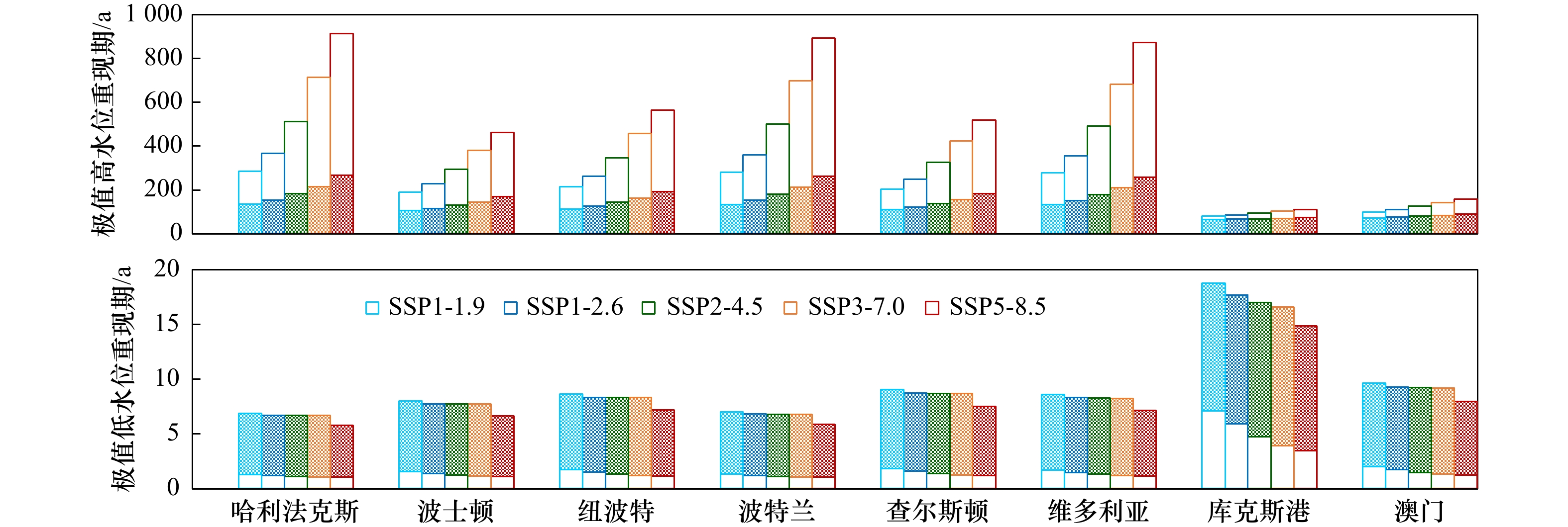
图 10 工程设计使用年限为50 a时各验潮站处不同方法推算的极值高、低水位在当前极值分布(2020年)中的重现期
白色填充部分由2020年极值高、低水位线性叠加工程设计使用年限内IPCC海平面上升预测值作为极值水位推算得到;阴影部分由采用本文构建方法、结合IPCC海平面上升预测计算的极值水位推算得到
Fig. 10 Return periods of extreme high and low water levels with the design lifetime of 50 a in the current extreme value distribution (the year of 2020) estimated by different methods
The white-filled area denotes the summation of extreme high/low water level and the predicted sea-level rise within the design lifetime of coastal facilities by IPCC; the shaded area denotes extreme high/low water level estimated by the method proposed in this study based on the predicted sea-level rise by IPCC

图 11 SSP5-8.5情景下澳门验潮站处不同工程设计使用年限相应极值高、低水位事件的年超越概率
Fig. 11 Exceedance probability of different return water levels for the Macao tide gauge station under the SSP5-8.5 green house gas emission scenario estimated by IPCC
表 1 验潮站及相应水位资料信息
Tab. 1 Tide gauge stations and the corresponding water level data information
序号 验潮站 位置 水位数据覆盖年限 水位数据序列长度/a 1 哈利法克斯(Halifax) 44.667°N, 63.583°W 1920–2013 94 2 波士顿(Boston) 42.353°N, 71.053°W 1922–2019 98 3 纽波特(Newport) 41.505°N, 71.327°W 1931–2019 89 4 波特兰(Portland) 43.657°N, 70.247°W 1912–2019 108 5 查尔斯顿(Charleston) 32.782°N, 79.925°W 1922–2019 98 6 维多利亚(Victoria) 48.417°N, 123.367°W 1909–2018 110 7 洛杉矶(Los Angeles) 33.720°N, 118.272°W 1924–2019 96 8 旧金山(San Francisco) 7.807°N, 122.465°W 1898–2016 119 9 库克斯港(Cuxhaven) 53.867°N, 8.717°E 1918–2018 101 10 澳门(Macao) 22.200°N, 113.550°E 1925–2017 93  下载: 导出CSV
表 2 62 a滑动时窗下各验潮站平均海平面与高、低水位位置参数的皮尔逊相关系数
Tab. 2 Pearson correlation coefficient of mean sea level and location parameters for the annual high and low water level with the 62 a running time window at the 10 tide gauge stations
验潮站 高水位位置参数 低水位位置参数 哈利法克斯(Halifax) 0.992 0 0.998 2 波士顿(Boston) 0.994 8 0.991 6 纽波特(Newport) 0.997 2 0.991 4 波特兰(Portland) 0.997 0 0.974 9 查尔斯顿(Charleston) 0.996 6 0.918 9 维多利亚(Victoria) 0.944 5 0.805 2 洛杉矶(Los Angeles) 0.984 8 0.814 1 旧金山(San Francisco) 0.995 6 0.985 4 库克斯港(Cuxhaven) 0.969 7 0.890 2 澳门(Macao) 0.978 5 0.966 5
下载: 导出CSV
表 3 62 a滑动时窗下各验潮站平均海平面和高、低水位位置参数线性上升速率
Tab. 3 Linear trends of mean sea-level and location parameters for the annual high and low water level with the 62 a running time window at the 10 tide gauge stations
验潮站 线性上升速率/(cm·a−1) 平均海平面 高水位位置参数 低水位位置参数 哈利法克斯(Halifax) 0.317 0.305 0.387 波士顿(Boston) 0.262 0.341 0.256 纽波特(Newport) 0.271 0.385 0.245 波特兰(Portland) 0.187 0.281 0.164 查尔斯顿(Charleston) 0.316 0.325 0.145 维多利亚(Victoria) 0.084 0.114 0.075 洛杉矶(Los Angeles) 0.085 0.072 0.047 旧金山(San Francisco) 0.200 0.247 0.148 库克斯港(Cuxhaven) 0.200 0.606 0.266 澳门(Macao) 0.163 0.319 0.217
下载: 导出CSV
表 4 各验潮站2020年高水位极值的耿贝尔分布拟合结果
Tab. 4 The fitting results of location parameters of Gumbel distribution in the year of 2020 for the annual high water level at the 10 tide gauge stations
参数验潮站 位置参数/cm 尺度参数/cm 极值水位/cm 25 a一遇 50 a一遇 80 a一遇 100 a一遇 哈利法克斯(Halifax) 234.4 12.0 272.8 281.2 286.9 289.6 波士顿(Boston) 496.6 15.7 546.8 557.9 565.3 568.8 纽波特(Newport) 233.5 14.4 279.6 289.7 296.5 299.7 波特兰(Portland) 634.0 12.1 672.7 681.2 686.9 689.7 查尔斯顿(Charleston) 311.4 14.9 359.1 369.5 376.6 379.9 维多利亚(Victoria) 330.3 12.2 369.3 377.9 383.7 386.4 洛杉矶(Los Angeles) 336.2 5.3 353.2 356.9 359.4 360.6 旧金山(San Francisco) 405.6 9.6 436.3 443.1 447.6 449.8 库克斯港(Cuxhaven) 837.0 44.2 978.4 1 009.5 1 030.4 1 040.3 澳门(Macao) 340.2 30.4 437.4 458.8 473.2 480.0
下载: 导出CSV
表 5 各验潮站2020年低水位极值的耿贝尔分布拟合结果
Tab. 5 The fitting results of location parameters of Gumbel distribution in the year of 2020 for the annual low water level at the 10 tide gauge stations
参数验潮站 位置参数/cm 尺度参数/cm 极值水位/cm 25 a一遇 50 a一遇 80 a一遇 100 a一遇 哈利法克斯(Halifax) –26.5 7.7 –35.5 –37.0 –37.9 –38.3 波士顿(Boston) 26.0 9.5 14.9 13.0 12.0 11.5 纽波特(Newport) –7.5 10.6 –19.9 –22.0 –23.2 –23.7 波特兰(Portland) 186.5 7.9 177.3 175.7 174.8 174.4 查尔斯顿(Charleston) 7.6 11.3 –5.6 –7.8 –9.1 –9.7 维多利亚(Victoria) –24.1 10.5 –36.4 –38.4 –39.6 –40.1 洛杉矶(Los Angeles) 57.0 4.9 51.3 50.3 49.8 49.5 旧金山(San Francisco) 119.5 6.7 111.7 110.4 109.6 109.3 库克斯港(Cuxhaven) 212.4 30.4 176.9 170.9 167.5 166.0 澳门(Macao) 28.4 12.3 14.0 11.6 10.2 9.6
下载: 导出CSV
-
[1] IPCC. Climate Change 2021: the Physical Science Basis. Contribution of Working Group I to the Sixth Assessment Report of the Intergovernmental Panel on Climate Change[M]. Cambridge: Cambridge University Press, 2021. [2] 中华人民共和国自然资源部. 2020年中国海平面公报[EB/OL]. (2021–04–21)[2022–03–28]. https://www.nmdis.org.cn/hygb/zghpmgb/.Ministry of Natural Resources, People's Republic of China. China sea level bulletin for the year of 2020[EB/OL]. (2021–04–21)[2022–03–28]. https://www.nmdis.org.cn/hygb/zghpmgb/. [3] 于宜法, 俞聿修. 海平面长期变化对推算多年一遇极值水位的影响[J]. 海洋学报, 2003, 25(3): 1−7.Yu Yifa, Yu Yuxiu. The effect of long-term sea-level variation on calculating the extreme water levels of multiyear return periods[J]. Acta Oceanologica Sinica, 2003, 25(3): 1−7. [4] Bernier N B, Thompson K R, Ou J, et al. Mapping the return periods of extreme sea levels: allowing for short sea level records, seasonality, and climate change[J]. Global and Planetary Change, 2007, 57(1/2): 139−150. [5] Hunter J. Estimating sea-level extremes under conditions of uncertain sea-level rise[J]. Climatic Change, 2010, 99(3): 331−350. [6] 于宜法, 刘兰, 郭明克, 等. 海平面变化和调和常数不稳定性对一些工程设计参数的影响[J]. 中国海洋大学学报(自然科学版), 2010, 40(6): 27−35.Yu Yifa, Liu Lan, Guo Mingke, et al. Influence of the mean-sea-level variation and harmonics instability on some design paramiters of engineering[J]. Periodical of Ocean University of China, 2010, 40(6): 27−35. [7] 于宜法, 刘兰, 李磊. 月平均海平面变化对设计水位的影响—推荐一种计算设计水位的方法[J]. 中国海洋大学学报(自然科学版), 2013, 43(9): 1−11.Yu Yifa, Liu Lan, Li Lei. The influence of monthly mean-sea-level variation on design water level: recommending a kind of method for calculating design water level[J]. Periodical of Ocean University of China, 2013, 43(9): 1−11. [8] Rashid M, Wahl T, Chambers D P, et al. An extreme sea level indicator for the contiguous United States coastline[J]. Scientific Data, 2019, 6(1): 326. doi: 10.1038/s41597-019-0333-x [9] Marcos M, Calafat F M, Berihuete Á, et al. Long-term variations in global sea level extremes[J]. Journal of Geophysical Research: Oceans, 2015, 120(12): 8115−8134. doi: 10.1002/2015JC011173 [10] Wahl T, Chambers D P. Evidence for multidecadal variability in US extreme sea level records[J]. Journal of Geophysical Research: Oceans, 2015, 120(3): 1527−1544. doi: 10.1002/2014JC010443 [11] Cid A, Menéndez M, Castanedo S, et al. Long-term changes in the frequency, intensity and duration of extreme storm surge events in southern Europe[J]. Climate Dynamics, 2016, 46(5): 1503−1516. [12] Mentaschi L, Vousdoukas M, Voukouvalas E, et al. The transformed-stationary approach: a generic and simplified methodology for non-stationary extreme value analysis[J]. Hydrology and Earth System Sciences, 2016, 20(9): 3527−3547. doi: 10.5194/hess-20-3527-2016 [13] Marcos M, Woodworth P L. Spatiotemporal changes in extreme sea levels along the coasts of the North Atlantic and the Gulf of Mexico[J]. Journal of Geophysical Research: Oceans, 2017, 122(9): 7031−7048. doi: 10.1002/2017JC013065 [14] Vousdoukas M I, Mentaschi L, Voukouvalas E, et al. Global probabilistic projections of extreme sea levels show intensification of coastal flood hazard[J]. Nature Communications, 2018, 9(1): 2360. doi: 10.1038/s41467-018-04692-w [15] Church J A, Hunter J R, McInnes K L, et al. Sea-level rise around the Australian coastline and the changing frequency of extreme events[J]. Australian Meteorological Magazine, 2006, 55(4): 253−260. [16] Lee H S. Estimation of extreme sea levels along the Bangladesh coast due to storm surge and sea level rise using EEMD and EVA[J]. Journal of Geophysical Research: Oceans, 2013, 118(9): 4273−4285. doi: 10.1002/jgrc.20310 [17] Talke S A, Orton P, Jay D A. Increasing storm tides in New York harbor, 1844–2013[J]. Geophysical Research Letters, 2014, 41(9): 3149−3155. doi: 10.1002/2014GL059574 [18] 庄圆, 纪棋严, 左军成, 等. 海平面上升对中国沿海地区极值水位重现期的影响[J]. 海洋科学进展, 2021, 39(1): 20−29. doi: 10.3969/j.issn.1671-6647.2021.01.003Zhuang Yuan, Ji Qiyan, Zuo Juncheng, et al. Effects of sea-level rise on the recurrence periods of extreme water levels in coastal areas of China[J]. Advances in Marine Science, 2021, 39(1): 20−29. doi: 10.3969/j.issn.1671-6647.2021.01.003 [19] Menéndez M, Woodworth P L. Changes in extreme high water levels based on a quasi-global tide-gauge data set[J]. Journal of Geophysical Research: Oceans, 2010, 115(C10): C10011. [20] Feng Xiangbo, Tsimplis M N. Sea level extremes at the coasts of China[J]. Journal of Geophysical Research: Oceans, 2014, 119(3): 1593−1608. doi: 10.1002/2013JC009607 [21] Haigh I D, Wadey M P, Wahl T, et al. Spatial and temporal analysis of extreme sea level and storm surge events around the coastline of the UK[J]. Scientific Data, 2016, 3(1): 160107. doi: 10.1038/sdata.2016.107 [22] Calafat F M, Wahl T, Tadesse M G, et al. Trends in Europe storm surge extremes match the rate of sea-level rise[J]. Nature, 2022, 603(7903): 841−845. doi: 10.1038/s41586-022-04426-5 [23] Coles S. An Introduction to Statistical Modeling of Extreme Values[M]. London: Springer, 2001. [24] Leadbetter M R, Lindgren G, Rootzén H. Extremes and Related Properties of Random Sequences and Processes[M]. New York: Springer-Verlag, 1983. [25] Hüsler J. Extreme values of non-stationary random sequences[J]. Journal of Applied Probability, 1986, 23(4): 937−950. doi: 10.2307/3214467 [26] Butler A, Heffernan J E, Tawn J A, et al. Extreme value analysis of decadal variations in storm surge elevations[J]. Journal of Marine Systems, 2007, 67(1/2): 189−200. [27] Calafat F M, Marcos M. Probabilistic reanalysis of storm surge extremes in Europe[J]. Proceedings of the National Academy of Sciences of the United States of America, 2020, 117(4): 1877−1883. doi: 10.1073/pnas.1913049117 [28] 史道济. 实用极值统计方法[M]. 天津: 天津科学技术出版社, 2006.Shi Daoji. Practical Methods for Extreme Value Statistics[M]. Tianjin: Tianjin Science and Technology Press, 2006. [29] Woodworth P L, Blackman D L. Evidence for systematic changes in extreme high waters since the mid-1970s[J]. Journal of Climate, 2004, 17(6): 1190−1197. doi: 10.1175/1520-0442(2004)017<1190:EFSCIE>2.0.CO;2 [30] Marcos M, Tsimplis M N, Shaw A G P. Sea level extremes in southern Europe[J]. Journal of Geophysical Research: Oceans, 2009, 114(C1): C01007. [31] Haigh I, Nicholls R, Wells N. Assessing changes in extreme sea levels: application to the English Channel, 1900–2006[J]. Continental Shelf Research, 2010, 30(9): 1042−1055. doi: 10.1016/j.csr.2010.02.002 [32] Tsimplis M N, Shaw A G P. Seasonal sea level extremes in the Mediterranean Sea and at the Atlantic European coasts[J]. Natural Hazards and Earth System Sciences, 2010, 10(7): 1457−1475. doi: 10.5194/nhess-10-1457-2010 [33] 中华人民共和国交通运输部. JTS 141−2011, 水运工程设计通则[S]. 北京: 人民交通出版社, 2011.Ministry of Transport of the People's Republic of China. JTS 141−2011, General rules for design of port and waterway works[S]. Beijing: China Communications Press, 2011. [34] 中华人民共和国交通运输部. JTS 145−2015, 港口与航道水文规范[S]. 北京: 人民交通出版社, 2016.Ministry of Transport of the People's Republic of China. JTS 145−2015, Code of hydrology for harbour and waterway[S]. Beijing: China Communications Press, 2016. [35] Benjamin J R, Cornell C A. Probability, Statistics, and Decision for Civil Engineers[M]. New York: McGraw Hill, 1970. [36] Salas J D, Obeysekera J. Revisiting the concepts of return period and risk for nonstationary hydrologic extreme events[J]. Journal of Hydrologic Engineering, 2014, 19(3): 554−568. doi: 10.1061/(ASCE)HE.1943-5584.0000820 [37] Du Tao, Xiong Lihua, Xu Chongyu, et al. Return period and risk analysis of nonstationary low-flow series under climate change[J]. Journal of Hydrology, 2015, 527: 234−250. doi: 10.1016/j.jhydrol.2015.04.041 [38] Shaw A G P, Tsimplis M N. The 18.6 yr nodal modulation in the tides of Southern European coasts[J]. Continental Shelf Research, 2010, 30(2): 138−151. doi: 10.1016/j.csr.2009.10.006 [39] Torres R R, Tsimplis M N. Tides and long-term modulations in the Caribbean Sea[J]. Journal of Geophysical Research: Oceans, 2011, 116(C10): C10022. doi: 10.1029/2011JC006973 [40] 黄琳, 孙佳, 杨逸秋, 等. 北太平洋海表面高度(SSH)与风应力变化的关系[J]. 海洋与湖沼, 2013, 44(1): 111−119. doi: 10.11693/hyhz201301017017Huang Lin, Sun Jia, Yang Yiqiu, et al. Sea surface height (SSH) change and its relationship with wind stress in the North Pacific Ocean[J]. Oceanologia et Limnologia Sinica, 2013, 44(1): 111−119. doi: 10.11693/hyhz201301017017 [41] 左军成, 左常圣, 李娟, 等. 近十年我国海平面变化研究进展[J]. 河海大学学报(自然科学版), 2015, 43(5): 442−449.Zuo Juncheng, Zuo Changsheng, Li Juan, et al. Advances in research on sea level variations in China from 2006 to 2015[J]. Journal of Hohai University (Natural Sciences), 2015, 43(5): 442−449. [42] Dixon M J, Tawn J A. The effect of non-stationarity on extreme sea-level estimation[J]. Journal of the Royal Statistical Society: Series C (Applied Statistics), 1999, 48(2): 135−151. doi: 10.1111/1467-9876.00145 [43] Devlin A T, Jay D A, Talke S A, et al. Coupling of sea level and tidal range changes, with implications for future water levels[J]. Scientific Reports, 2017, 7(1): 17021. doi: 10.1038/s41598-017-17056-z [44] Oey L Y, Chou S. Evidence of rising and poleward shift of storm surge in western North Pacific in recent decades[J]. Journal of Geophysical Research: Oceans, 2016, 121(7): 5181−5192. doi: 10.1002/2016JC011777 [45] Feng Xingru, Li Mingjie, Yin Baoshu, et al. Study of storm surge trends in typhoon-prone coastal areas based on observations and surge-wave coupled simulations[J]. International Journal of Applied Earth Observation and Geoinformation, 2018, 68: 272−278. doi: 10.1016/j.jag.2018.01.006 [46] Ray R D, Egbert G D, Erofeeva S Y. Tide predictions in shelf and coastal waters: status and prospects[M]//Vignudelli S, Kostianoy A G, Cipollini P, et al. Coastal Altimetry. Berlin, Heidelberg: Springer, 2011: 191−216. -

计量
- 文章访问数: 799
- HTML全文浏览量: 297
- PDF下载量: 109
- 被引次数: 0
