

Identification of hard-thin layers on the seabed or shallow sediments using geophysical data: A case study in the Liwan pipeline route, northern South China Sea
-
摘要: 由沉溺珊瑚礁、各类胶结砂以及胶结的珊瑚石或贝壳碎屑等组成的硬质薄层通常呈零散状分布,地质取样难以准确确定它们是如何分布的,这给海底管线施工带来极大的困难和风险。本文以南海北部为例,基于多种物探资料并结合正演模拟,分析、总结了海底以及海底之下硬质薄层的声学特征,在研究区综合识别出23个硬质薄层分布区。研究认为,硬质薄层与松散沉积物物理性质的差异可用于声学探测数据识别和定位。在浅地层剖面上,硬质薄层表现为强反射薄层,并对其下方地层的地震反射信号有一定的屏蔽作用,这一现象有助于确定硬质薄层是否存在以及其埋深和位置。在侧扫声呐影像和后向散射强度图上,硬质薄层通常表现为具有不规则形状的明暗变化阴影,阴影的边界指示了硬质薄层的分布范围。当硬质薄层出露于海底时,侧扫影像、反向散射强度结合浅地层剖面可以有效地识别并确定硬质薄层的范围;而当硬质薄层位于海床浅部(埋深数米到十几米)时,浅地层剖面可能是识别硬质薄层的唯一且最有效的方法。Abstract: The hard-thin layers (HTLs) are usually composed of submerged coral reefs, various cemented sands, cemented coral stones or shell fragments and their locations are difficult to be determined by geological sampling due to their sporadic distribution. They bring great challenges and risks to the construction of submarine pipelines. In this paper, taking the northern shelf of the South China Sea as an example, we summarized the acoustic characteristics of the HTLs on the seabed and in the shallow sediments based on a variety of high-resolution geophysical data combined with forward simulation analysis. Twenty-three areas with HTLs in the study area were determined. Our study suggests that differences in the physical properties of HTLs and loose sediments help identify and locate them using high-resolution geophysical data. On the sub-bottom profiles, the HTLs are characterized by reflective interfaces with high-amplitude, beneath of which the low-amplitude reflections usually occur. These reflection features help to determine the HTLs, their depths and locations. The HTLs usually display the alternating light and dark zones with irregular boundaries on the side scan sonar and backscatter intensity images. When the HTLs are located on the seafloor, the comprehensive interpretation of the side-scan images, backscatter intensity images and the sub-bottom profiles is effective to identify and locate them. For those THLs several meters to ten meters below the seafloor, high-resolution sub-bottom profiles may be the only and most effective way to identify and locate them.
-
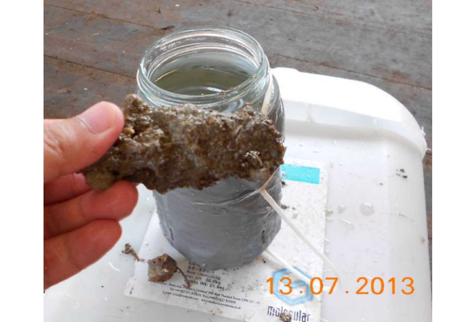
图 1 南海北部陆架路由区取样中的珊瑚石照片
Fig. 1 Photo of coral rocks in geological samples in the route area of northern shelf of the South China Sea
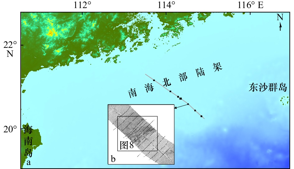
图 2 研究中收集的工程物探资料分布
a中灰色线表示侧扫声呐和多波束数据覆盖的条带状区域,黑色点表示有浅地层剖面数据的区域,其中一个区域进行了放大如b
Fig. 2 Track of geophysical data collected in the study area
Grey lines represent the narrow zone covered by side-scan sonar and multibeam data and black dots represent the areas with sub-bottom profiles in a. An area is enlarged as in b
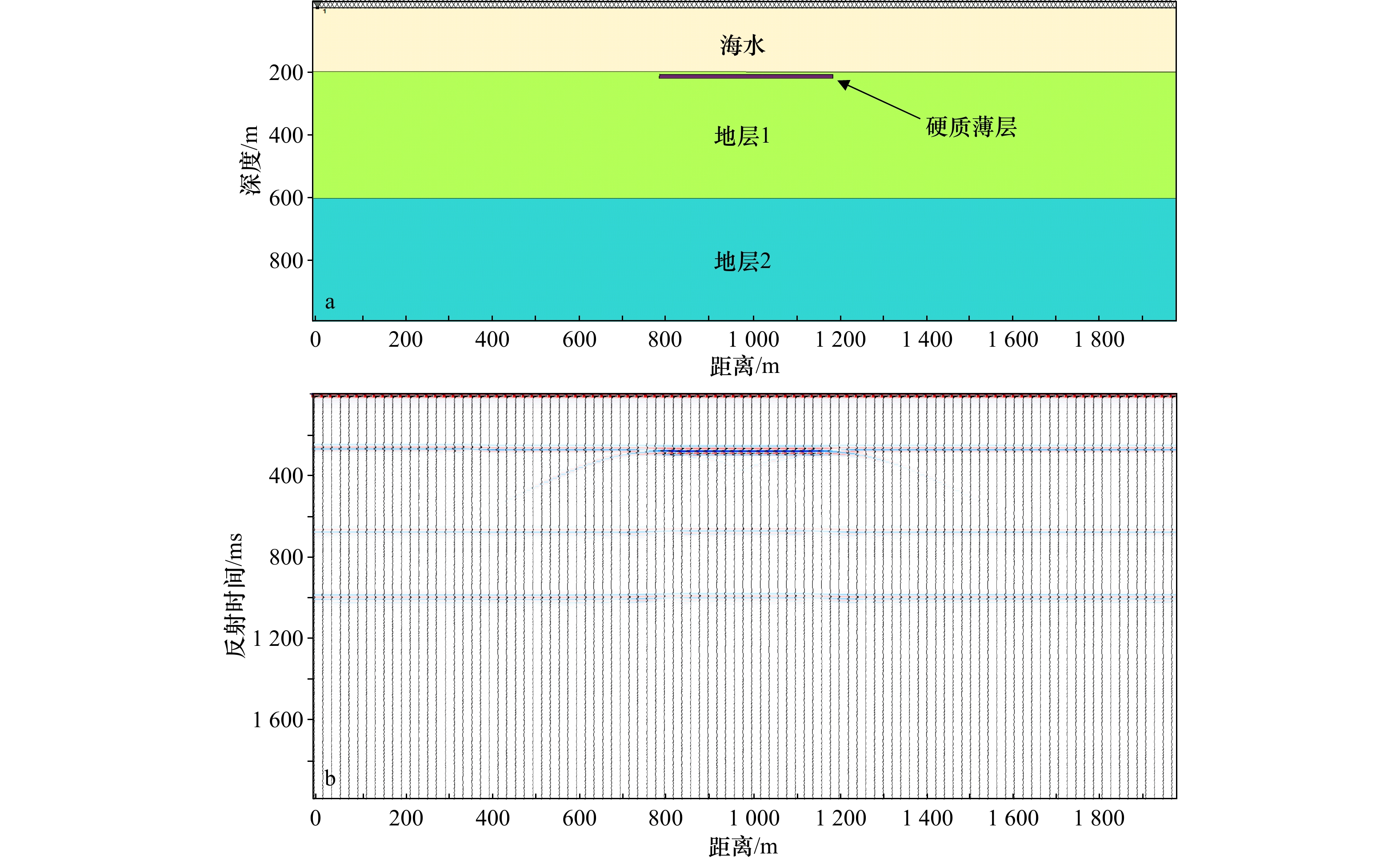
图 3 模型I(a)及地震正演结果(b)
模型I中不同介质(硬质薄层、海水、地层1和地层2)的密度取值相同,仅考虑速度差异而引起的波阻抗变化,硬质薄层纵波波速取3 000 m/s,海水波纵波波速取1 500 m/s,地层1纵波波速取 2 000 m/s,地层2纵波波速取2 500 m/s
Fig. 3 Model I (a) and seismic forward result (b)
In model I, the density of medias (hard-thin layer, seawater, formation 1 and formation 2) are assumed to be same; therefore, impedances of the medias are determined by their sound velocities. Here, the sound velocity is taken as 3 000 m/s for the hard-thin layer, 1 500 m/s for seawater, 2 000 m/s for formation 1 and 2 500 m/s for formation 2
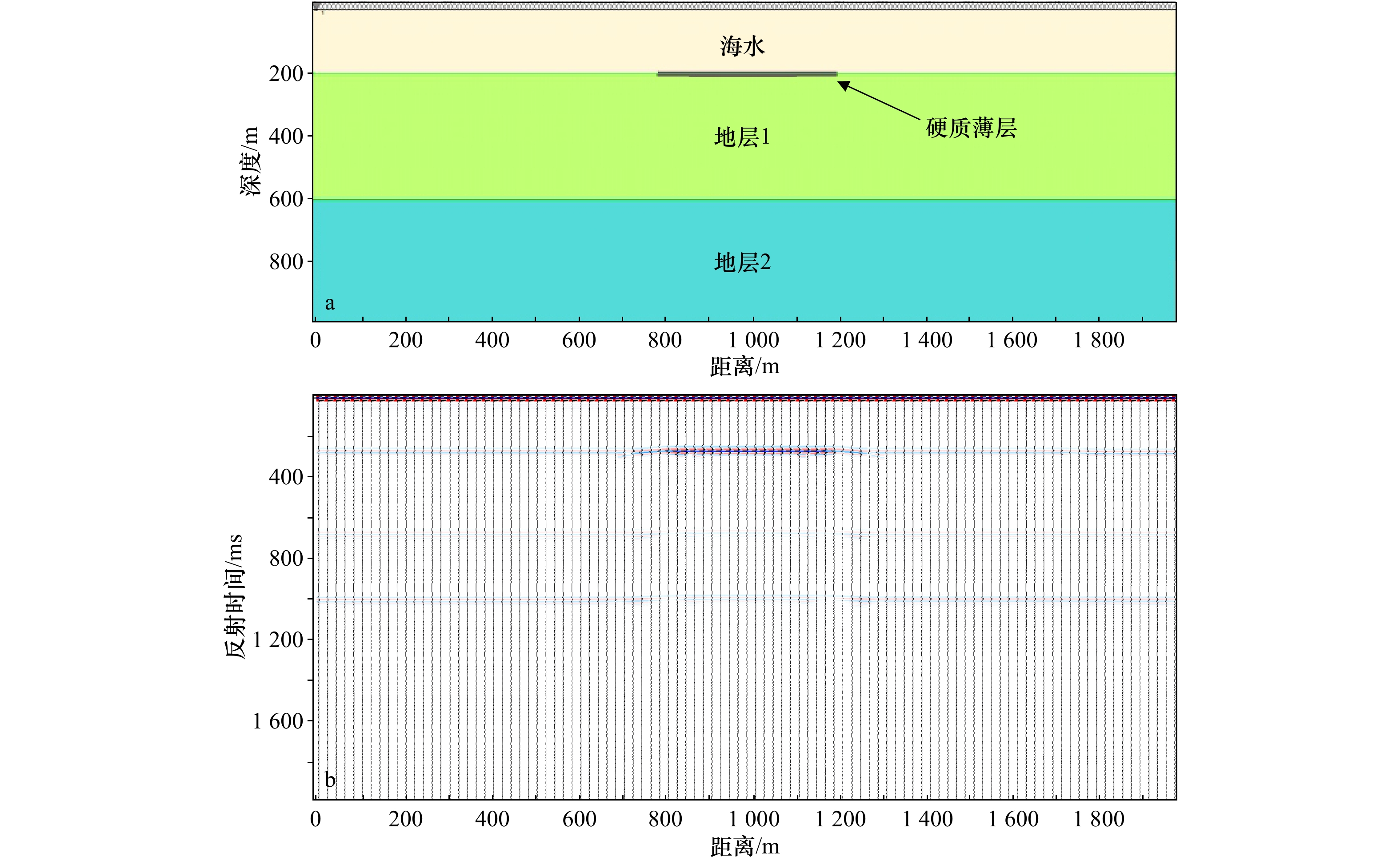
图 4 模型II(a)及地震正演结果(b)
模型II中不同介质(硬质薄层、海水、地层1和地层2)的密度取值相同,仅考虑速度差异而引起的波阻抗变化,硬质薄层纵波波速取3 000 m/s,海水波纵波波速取1 500 m/s,地层1纵波波速取 2 000m/s,地层2纵波波速取2 500 m/s
Fig. 4 Model II (a) and seismic forward result (b)
In model II, the density of medias (hard-thin layer, seawater, formation 1 and formation 2) are assumed to be same; therefore, impedances of the medias are determined by their sound velocities. Here, the sound velocity is taken as 3 000 m/s for the hard-thin layer 1 500 m/s for seawater, 2 000 m/s for formation 1 and 2 500 m/s for formation 2
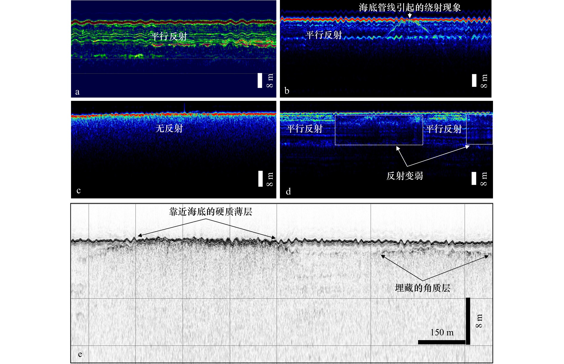
图 5 路由区典型声学反射相(a−d)以及陆架外缘的埋藏硬质薄层反射特征(e)
a. 振幅较强的平行反射;b. 振幅较弱的平行反射及管线引起的绕射;c. 海底下方的无反射;d. 强反射海底下反射突然变弱现象
Fig. 5 Typical acoustic reflection facies (a−d) in the study area and the reflection configuration of the buried hard-thin layers at the outer edge of the shelf (e)
a. Parallel reflections with high amplitude; b. parallel reflections with low amplitude and diffractions caused by the pipeline; c. no reflections beneath the seafloor; d. the phenomenon that amplitude of the reflections are abruptly lower beneath the seafloor which has high-amplitude reflections
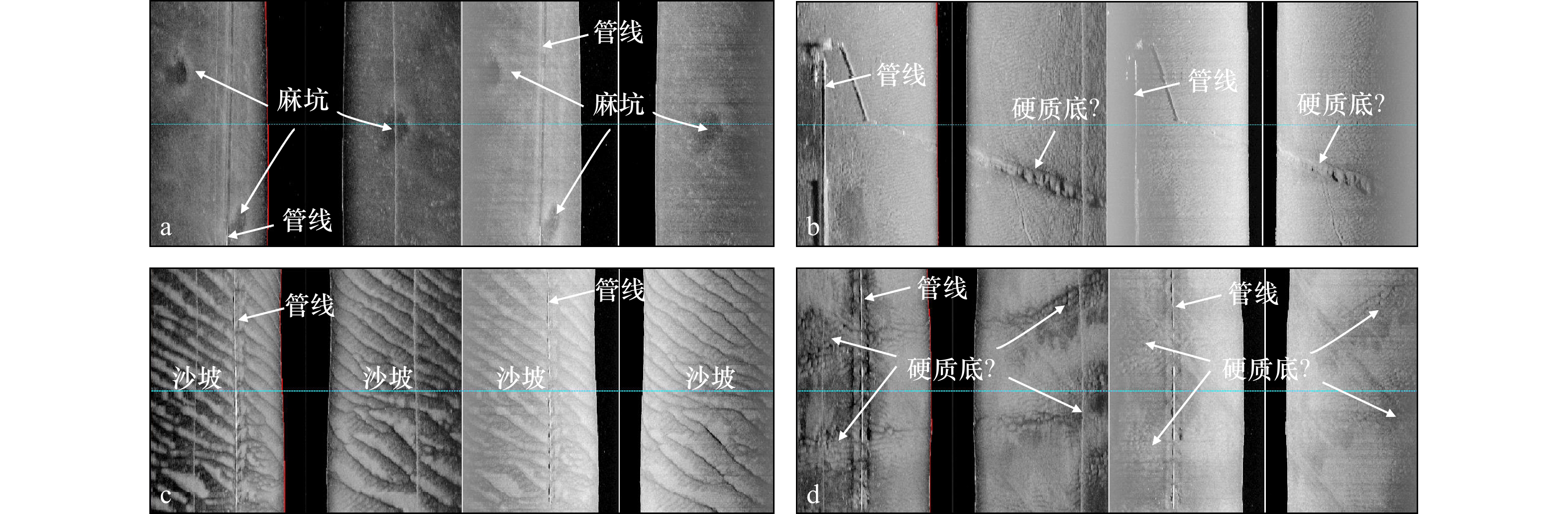
图 6 侧扫声呐影像揭示的典型地貌(a−d中左侧影像为高频,右侧为低频)
Fig. 6 Typical geomorphological features revealed by side-scan sonar images (left images in a−d were acquired with high frequencies and right ones were acquired with low frequencies)

图 7 后向散射强度灰度图揭示的典型地貌
Fig. 7 Typical geomorphological features revealed by the grayscale map of backscatter intensity

图 8 多种物探资料解释的硬质薄层
a 为侧扫声呐影像,b 为后向散射强度,c 为浅地层剖面。a 和 b 中红色虚线圈定的区域为硬质薄层分布区;c 中带双箭头的白线为硬质薄层的分布区
Fig. 8 Comprehensive interpretation of hard-thin layers by geophysical data
a is sde-scan sonar image, b is backscattering intensity and c is sub-bottom profile. The area delineated by the red dotted lines is the distribution area of the hard-thin layers in a and b. The white lines with double arrows indicate the distribution of the hard-thin layers in c
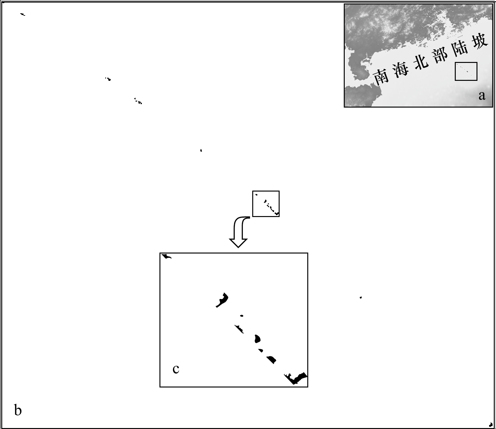
图 9 研究区内识别的硬质薄层的分布(埋藏深度小于5 m)
b的位置见右上角a;c是b的局部放大,黑色区域为识别的硬质薄层分布区
Fig. 9 The location of hard-thin layers (buried depth is less than 5 m) identified in the study area
The location of b is shown in a, and c is a partial enlargement of b. Black areas denote the distribution area of hard-thin layers identified by geophysical data
表 1 地震正演模型参数
Tab. 1 Parameters in seismic forward models
模型 I 模型 II 硬质薄层宽度 400 m 400 m 硬质薄层厚度 10 m 10 m 硬质薄层位置 海底以下10 m 出露海底5 m  下载: 导出CSV
-
[1] 吴海京, 年永吉. 南海东部几种典型海底地貌特征的研究与认识[J]. 地球物理学进展, 2017, 32(2): 919−926. doi: 10.6038/pg20170264Wu Haijing, Nian Yongji. Research and cognition for several typical seabed features in the eastern of the South China Sea[J]. Progress in Geophysics, 2017, 32(2): 919−926. doi: 10.6038/pg20170264 [2] Li Xishuang, Li Xinzhong, Zhao Qiang, et al. The occurrence, acoustic characteristics, and significance of submerged reefs on the continental shelf edge and upper slope, northern South China Sea[J]. Continental Shelf Research, 2015, 100: 11−24. doi: 10.1016/j.csr.2015.03.006 [3] 王琳. 乐东22-1/15-1油气管线路由区工程地质灾害研究[D]. 青岛: 中国海洋大学, 2007, 17-19.Wang Lin. Research on the hazards of engineering geology about the route of Ledong 22-1/15-1 proposed pipeline[D]. Qingdao: Ocean University of China, 2007: 17−19. [4] 陈岱新, 郝高建, 王涛, 等. 莺歌海中部区域硬质海底特征及其工程影响[J]. 海洋地质前沿, 2016, 32(9): 47−52, 63. doi: 10.16028/j.1009-2722.2016.09007Chen Daixin, Hao Gaojian, Wang Tao, et al. Characteristics of hard seafloor in central Yinggehai and its engineering significance[J]. Marine Geology Frontiers, 2016, 32(9): 47−52, 63. doi: 10.16028/j.1009-2722.2016.09007 [5] 徐梓辰, 金衍, 洪国斌, 等. 基于近钻头振动数据的海底硬质地层探测方法[J]. 船海工程, 2019, 48(4): 112−116. doi: 10.3963/j.issn.1671-7953.2019.04.025Xu Zichen, Jin Yan, Hong Guobin, et al. Detection method of seabed hard strata based on near-bit vibration data[J]. Ship & Ocean Engineering, 2019, 48(4): 112−116. doi: 10.3963/j.issn.1671-7953.2019.04.025 [6] Jackson D R, Richardson M D. High-Frequency Seafloor Acoustics[M]. New York: Springer, 2007: 131−142. [7] Berkovitch A, Belfer I, Hassin Y, et al. Diffraction imaging by multifocusing[J]. Geophysics, 2009, 74(6): WCA75−WCA81. doi: 10.1190/1.3198210 [8] Lee S H, Kim K H. Side-scan sonar characteristics and manganese nodule abundance in the clarion-clipperton fracture zones, NE equatorial Pacific[J]. Marine Georesources & Geotechnology, 2004, 22(1/2): 103−114. [9] 潘国富, 付晓明, 荀诤慷, 等. 侧扫声纳在海底光缆维护工程中的应用[J]. 工程地球物理学报, 2004, 1(5): 389−394. doi: 10.3969/j.issn.1672-7940.2004.05.001Pan Guofu, Fu Xiaoming, Xu Zhengkang, et al. Side scan sonar applications in undersea fiber-optic cable maintenance projects[J]. Chinese Journal of Engineering Geophysics, 2004, 1(5): 389−394. doi: 10.3969/j.issn.1672-7940.2004.05.001 [10] Collier J S, Humber S R. Time-lapse side-scan sonar imaging of bleached coral reefs: a case study from the Seychelles[J]. Remote Sensing of Environment, 2007, 108(4): 339−356. doi: 10.1016/j.rse.2006.11.029 [11] Kumagai H, Tsukioka S, Yamamoto H, et al. Hydrothermal plumes imaged by high-resolution side-scan sonar on a cruising AUV, Urashima[J]. Geochemistry, Geophysics, Geosystems, 2010, 11(12): Q12013. [12] Hogan K A, Dowdeswell J A, Mienert J, et al. New insights into slide processes and seafloor geology revealed by side-scan imagery of the massive Hinlopen slide, Arctic Ocean margin[J]. Geo-Marine Letters, 2013, 33(5): 325−343. doi: 10.1007/s00367-013-0330-6 [13] Bryant R S. Side scan sonar for hydrography-an evaluation by the Canadian hydrographic service[J]. The International Hydrographic Review, 2015, 52(1): 43−56. [14] Powers J, Brewer S K, Long J M, et al. Evaluating the use of side-scan sonar for detecting freshwater mussel beds in turbid river environments[J]. Hydrobiologia, 2015, 743(1): 127−137. doi: 10.1007/s10750-014-2017-z [15] 王晓, 王爱学, 蒋廷臣, 等. 侧扫声呐图像应用领域综述[J]. 测绘通报, 2019(1): 1−4. doi: 10.13474/j.cnki.11-2246.2019.0001Wang Xiao, Wang Aixue, Jiang Tingchen, et al. Review of application areas for side scan sonar image[J]. Bulletin of Surveying and Mapping, 2019(1): 1−4. doi: 10.13474/j.cnki.11-2246.2019.0001 [16] 周兴华, 姜小俊, 史永忠. 侧扫声纳和浅地层剖面仪在杭州湾海底管线检测中的应用[J]. 海洋测绘, 2007, 27(4): 64−67. doi: 10.3969/j.issn.1671-3044.2007.04.019Zhou Xinghua, Jiang Xiaojun, Shi Yongzhong. Application of side scan sonar and sub-bottom profile in the checking of submerged pipeline in Hangzhou Bay[J]. Hydrographic Surveying and Charting, 2007, 27(4): 64−67. doi: 10.3969/j.issn.1671-3044.2007.04.019 [17] 董庆亮, 欧阳永忠, 陈岳英, 等. 侧扫声纳和多波束测深系统组合探测海底目标[J]. 海洋测绘, 2009, 29(5): 51−53. doi: 10.3969/j.issn.1671-3044.2009.05.015Dong Qingliang, Ouyang Yongzhong, Chen Yueying, et al. Measuring bottom of sea target with side scan sonar and multibeam sounding system[J]. Hydrographic Surveying and Charting, 2009, 29(5): 51−53. doi: 10.3969/j.issn.1671-3044.2009.05.015 [18] 年永吉, 朱友生, 陈强, 等. 流花深水区块典型滑坡特征的研究与认识[J]. 地球物理学进展, 2014, 29(3): 1412−1417. doi: 10.6038/pg20140357Nian Yongji, Zhu Yousheng, Chen Qiang, et al. The research and cognition of typical submarine landslide characteristics of Liuhua deepwater block[J]. Progress in Geophysics, 2014, 29(3): 1412−1417. doi: 10.6038/pg20140357 [19] 卢胜周, 彭华, 马秀敏, 等. 侧扫声呐在琼州海峡跨海通道工程物探中的应用[J]. 地质论评, 2015, 61(S1): 89−90.Lu Shengzhou, Peng Hua, Ma Xiumin, et al. Application of side-scan sonar in geophysical prospecting of Qiongzhou Strait cross-sea channel engineering[J]. Geological Review, 2015, 61(S1): 89−90. [20] Degraer S, Moerkerke G, Rabaut M, et al. Very-high resolution side-scan sonar mapping of biogenic reefs of the tube-worm Lanice conchilega[J]. Remote Sensing of Environment, 2008, 112(8): 3323−3328. doi: 10.1016/j.rse.2007.12.012 [21] Clarke J E H, Mayer L A, Wells D E. Shallow-water imaging multibeam sonars: A new tool for investigating seafloor processes in the coastal zone and on the continental shelf[J]. Marine Geophysical Researches, 1996, 18(6): 607−629. doi: 10.1007/BF00313877 [22] Hewitt A, Salisbury R, Wilson J. Using multibeam echosounder backscatter to characterize seafloor features[J]. Sea Technology, 2010, 51(9): 10−13. [23] Brown C J, Todd B J, Kostylev V E, et al. Image-based classification of multibeam sonar backscatter data for objective surficial sediment mapping of Georges Bank, Canada[J]. Continental Shelf Research, 2011, 31(2): S110−S119. doi: 10.1016/j.csr.2010.02.009 [24] Hamilton L J, Parnum I. Acoustic seabed segmentation from direct statistical clustering of entire multibeam sonar backscatter curves[J]. Continental Shelf Research, 2011, 31(2): 138−148. doi: 10.1016/j.csr.2010.12.002 [25] Micallef A, Le Bas T P, Huvenne V A I, et al. A multi-method approach for benthic habitat mapping of shallow coastal areas with high-resolution multibeam data[J]. Continental Shelf Research, 2012, 39−40: 14−26. doi: 10.1016/j.csr.2012.03.008 [26] McGonigle C, Grabowski J H, Brown C J, et al. Detection of deep water benthic macroalgae using image-based classification techniques on multibeam backscatter at Cashes Ledge, Gulf of Maine, USA[J]. Estuarine, Coastal and Shelf Science, 2011, 91(1): 87−101. doi: 10.1016/j.ecss.2010.10.016 [27] Yang Yong, He Gaowen, Ma Jinfeng, et al. Acoustic quantitative analysis of ferromanganese nodules and cobalt-rich crusts distribution areas using EM122 multibeam backscatter data from deep-sea basin to seamount in western Pacific Ocean[J]. Deep-Sea Research Part I: Oceanographic Research Papers, 2020, 161: 103281. doi: 10.1016/j.dsr.2020.103281 [28] De Beukelaer S M, MacDonald I R, Guinnasso Jr N L, et al. Distinct side-scan sonar, RADARSAT SAR, and acoustic profiler signatures of gas and oil seeps on the Gulf of Mexico slope[J]. Geo-Marine Letters, 2003, 23(3/4): 177−186. [29] Lafferty B, Quinn R, Breen C. A side-scan sonar and high-resolution chirp sub-bottom profile study of the natural and anthropogenic sedimentary record of lower lough erne, northwestern Ireland[J]. Journal of Archaeological Science, 2006, 33(6): 756−766. doi: 10.1016/j.jas.2005.10.007 [30] Nakamura K, Toki T, Mochizuki N, et al. Discovery of a new hydrothermal vent based on an underwater, high-resolution geophysical survey[J]. Deep-Sea Research Part I: Oceanographic Research Papers, 2013, 74: 1−10. doi: 10.1016/j.dsr.2012.12.003 -

计量
- 文章访问数: 603
- HTML全文浏览量: 311
- PDF下载量: 46
- 被引次数: 0
