留言板

尊敬的读者、作者、审稿人, 关于本刊的投稿、审稿、编辑和出版的任何问题, 您可以本页添加留言。我们将尽快给您答复。谢谢您的支持!

姓名
邮箱
手机号码
标题
留言内容
验证码

渤海湾M2分潮的季节变化:增强调和分析的应用

余鹰 王道胜

余鹰,王道胜. 渤海湾M2分潮的季节变化:增强调和分析的应用[J]. 海洋学报,2021,43(5):1–13 doi: 10.12284/hyxb2021063
引用本文: 余鹰,王道胜. 渤海湾M2分潮的季节变化:增强调和分析的应用[J]. 海洋学报,2021,43(5):1–13 doi: 10.12284/hyxb2021063
Yu Ying,Wang Daosheng. Seasonal variability of the M2 constituent in the Bohai Bay: Application of enhanced harmonic analysis[J]. Haiyang Xuebao,2021, 43(5):1–13 doi: 10.12284/hyxb2021063
Citation: Yu Ying,Wang Daosheng. Seasonal variability of the M2 constituent in the Bohai Bay: Application of enhanced harmonic analysis[J]. Haiyang Xuebao,2021, 43(5):1–13 doi: 10.12284/hyxb2021063

渤海湾M2分潮的季节变化:增强调和分析的应用

doi: 10.12284/hyxb2021063
基金项目: 广东省重点领域研发计划(2020B1111020005);广东省基础与应用基础研究基金(2020A1515110339);深圳市基础研究资助项目(JCYJ20200109110220482)
详细信息
    作者简介:

    余鹰(1995—),男,湖北省云梦县人,主要从事数据分析、潮汐变化特征研究。E-mail:yuying6d1p@163.com

    通讯作者:

    王道胜,硕士生导师,副教授,主要从事浅海动力学、数据同化研究。E-mail:dswangouc@163.com

  • 中图分类号: P722.4

Seasonal variability of the M2 constituent in the Bohai Bay: Application of enhanced harmonic analysis

  • 摘要: M2分潮的季节变化对沿海的海洋环境有着重要影响。增强调和分析(EHA)既可以提取主要分潮时变的振幅和迟角,同时可以得到其他分潮不随时间变化的振幅和迟角。本文利用EHA分析渤海湾两个站点的水位数据,研究了渤海湾M2分潮的季节变化。为了评估EHA方法的准确性,在理想实验中设计了人造“水位数据”。利用EHA分析得到的M2分潮时变振幅和迟角以及S2、K1、O1分潮不随时间变化的振幅和迟角均比其他方法得到的结果更接近给定值,表明了EHA的有效性和可用性。当使用EHA分析渤海湾实际海平面观测数据时,得到的M2分潮振幅具有明显的季节变化特征:夏季较大,冬季较小。敏感性实验表明,分析所得渤海湾M2分潮振幅的季节变化趋势不受实验设置的影响,是鲁棒的,能够反映该海域真实的M2分潮季节变化。此外,渤海湾M2分潮振幅的季节变化可能是东亚季风通过影响平均海平面、层化和涡动黏性系数的季节变化而引起的。
  • 由于海洋物理性质和海岸形态的变化,潮汐存在多个时间尺度的变化[1],尤其是沿海和极地地区的M2分潮[2]。前人研究表明,英国海岸[3]、西北欧大陆架[4]、黄海和东海[5]、哈得孙河口[6]和东南亚海岸[1]等沿海地区,M2分潮都存在着季节变化。此外,相关研究表明极地地区M2分潮也存在季节变化[2, 7-8]

    为了分析M2分潮的季节变化,传统上将观测的水位数据分段,并对每一段进行经典调和分析(Classical Harmonic Analysis, CHA),该方法可以通过MATLAB中的T_TIDE工具包来实现[9]。上述过程称为分段调和分析(Segmented Harmonic Analysis, SHA),该方法在前人研究中得到广泛使用[2, 5, 10-13]。当直接使用SHA时,得到的振幅和迟角是离散的,需要对其进行插值以得到连续的结果。如果采用时间窗滑动的方式,一些峰值和快速变化的信号会被平滑,若某些分段中存在较多缺测,则可能导致计算结果不准确。除此之外,在使用SHA进行月度分析时,一些无法分辨的潮汐成分也需谨慎处理。Jin等[10]提出了增强调和分析(Enhanced Harmonic Analysis, EHA)方法,可以直接得到内潮不同潮汐成分时变的振幅和迟角。Pan等[14]基于EHA方法开发了S_TIDE工具包,并利用S_TIDE研究了哥伦比亚河口的潮汐−河流相互作用。根据Pan等[14]所述,在S_TIDE中如何针对分析的潮汐成分选择合适的独立点数是一项相对复杂的工作,应通过一系列敏感性试验来测试,以避免产生虚假的结果。

    在SHA和EHA中,所有潮汐成分的调和常数均被认为是随时间变化的。然而,潮汐季节变化的原因错综复杂[15],在大多数情况下,只有主要分潮(如M2分潮)的时间变化是显著并需要关注的,而其他分潮的时间变化比较微弱且可以忽略不计。EHA认为所有分潮的振幅和迟角都是随时间变化的,一方面增加了计算的复杂度和需要的计算机内存,另一方面显著减少了能够分辨的分潮数量。Wang等[16]对EHA进行了改进,使其不仅能得到主要分潮时变的振幅和迟角,同时也能得到其他分潮不变的振幅和迟角。为便于对EHA改进前后的效果进行对比分析,改进前的EHA,即:假定所有潮汐成分的调和常数均随时间变化的EHA,被记为OEHA(Original EHA),而改进后的EHA则简记为EHA。本文使用渤海湾的水位观测数据,通过设计理想实验,构建人造“水位数据”验证EHA的可行性和有效性,并利用EHA得到了渤海湾M2分潮振幅的季节变化,同时讨论了渤海湾M2分潮振幅季节变化的原因。

    海平面高度由多个因素决定,可表达为[16-18]

    $$\zeta (t) = {\zeta _0} + {\zeta _{{\rm{tide}}}}(t) + {\zeta _{{\rm{meteorology}}}}(t),$$ (1)

    式中,$\zeta (t)$代表海平面高度(即:水位),右边3项分别是平均海平面高度(Mean Sea Level, MSL)、潮汐引起的海表面高度、气象因素导致的海表面高度。在不考虑节点调制的情况下,潮汐的计算通常是k个分潮之和,即

    $${\zeta _{{\rm{tide}}}}(t) = \sum\limits_k {{a_k}\cos ({\omega _k}t - {\varphi _k})} ,$$ (2)

    式中,$\omega $$a$$\varphi $分别代表每个分潮的角速度(单位:rad/s),振幅(单位:m)和迟角(单位:rad)。在OEHA中,${\zeta _0}$$a$$\varphi $均被认为是随时间变化的[10, 14],即

    $$\begin{split} \zeta (t) &= {\zeta _0}(t) + {\zeta _{{\rm{tide}}}}(t) \\ & = {\zeta _0}(t) + \sum\limits_i {\left\{ {{a_i}(t) \cdot \cos \left[ {{\omega _i}t - {\varphi _i}(t)} \right]} \right\}} \end{split}. $$ (3)

    在OEHA的基础上,Wang等[16]进行了改进。在改进后的EHA中,只有几个主要分潮的振幅和迟角是时变的,而其他分潮的振幅和迟角仍然是常数[16]。因此,海平面高度的表达式为

    $$\begin{split} \zeta (t) =& {\zeta _0}(t) + {\zeta _{{\rm{tide}}}}(t) \\ =& {\zeta _0}(t) + \sum\limits_i {\left\{ {{a_i}(t) \cdot \cos \left[ {{\omega _i}t - {\varphi _i}(t)} \right]} \right\}} + \\ & \sum\limits_j {[{a_j} \cdot } \cos ({\omega _j}t - {\varphi _j})], \end{split} $$ (4)

    式中,具有时变振幅和迟角的分潮数量为i, 而振幅和迟角是常数的分潮数量为j${\zeta _0}\left( t \right)$包含气象因素导致的海表面高度[16]。类似于Jin等[10]和Pan等[14],改进后的EHA在求解时变的平均海平面高度、振幅和迟角时,引入了独立点方案和三次样条插值法,而上述的时变量和等号右边第三项中的常数振幅和迟角可以用最小二乘法同时求解。此外,误差评估算法与Jin等[10]和Pan等[14]相同。改进后的EHA已更新到S_TIDE中,可以从以下网站获取:https://www.researchgate.net/project/A-non-stationary-tidal-analysis-toolbox-S-TIDE

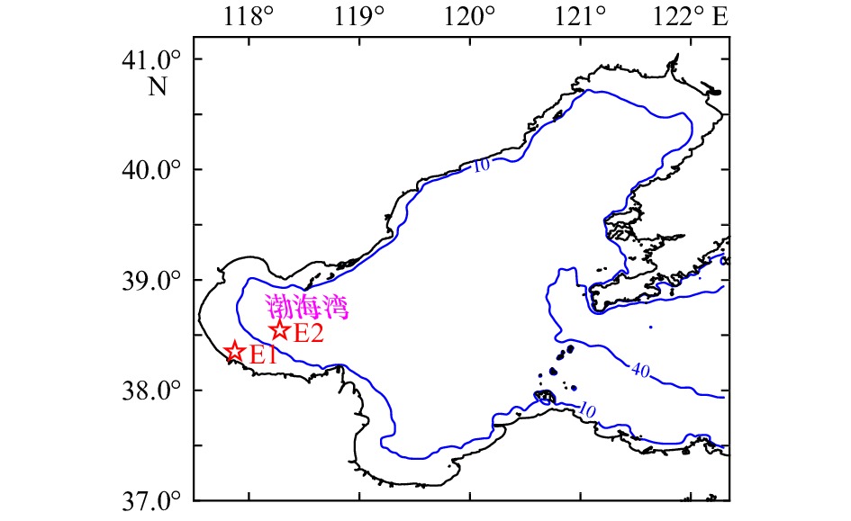
    本文采用的数据是中国渤海湾的两个站点E1和E2的逐时水位数据(已减去平均水位),观测数据的时间跨度为2013年11月1日(世界时,下同)到2014年11月1日,图1标注了E1和E2站点的位置。如图2所示,E1站点有大约1/4的数据缺测,而E2站点的数据是连续的,E1和E2的海平面振幅大多小于2 m。

    图  1  渤海湾观测站E1和E2的位置(红星),以及10 m和40 m水深线
    Figure  1.  The locations of the observation stations (E1 and E2, red stars) in the Bohai Bay, and the isobathymetric lines at 10 m and 40 m
    图  2  E1(a)和E2(b)站的水位观测数据
    洋红色实线描述了观测的时间段
    Figure  2.  The observed sea level at E1(a) and E2(b) stations
    The magenta solid lines describe the temporal locations of the observations

    在分析实际水位数据时,分潮振幅和迟角的真实值并不清楚,无法验证方法的准确性。因此,本文首先通过理想实验来验证EHA方法的可行性和有效性。

    2.3.1   人造“水位数据”

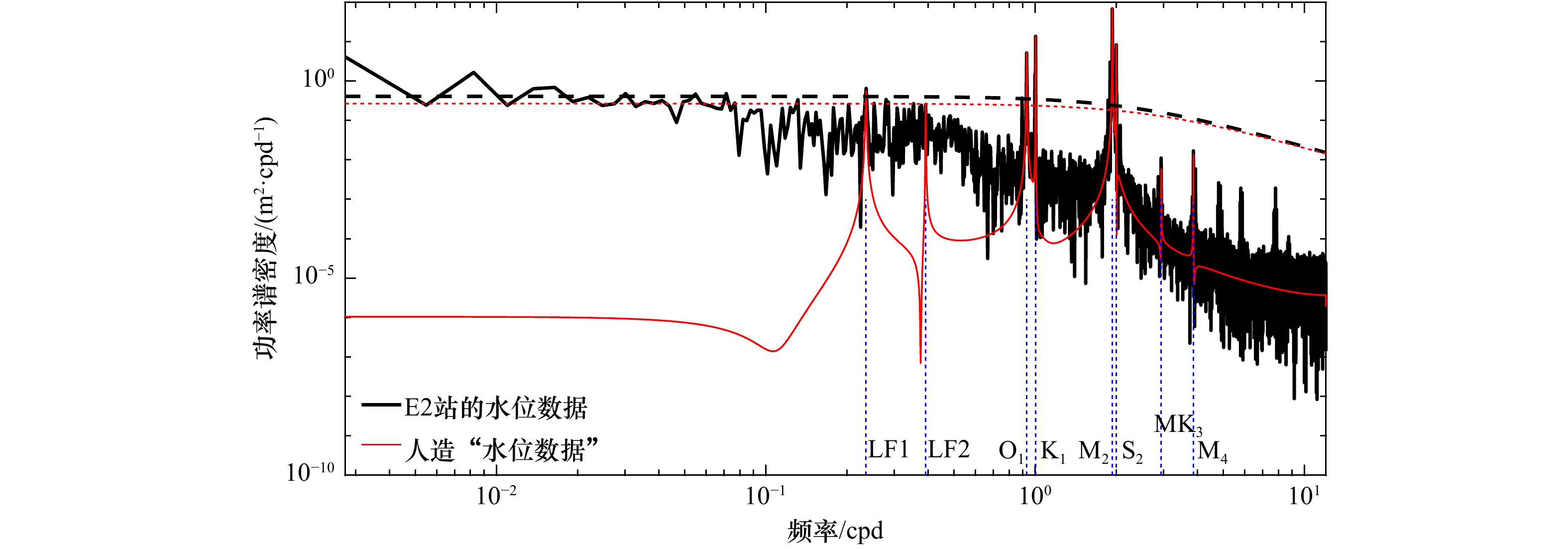
    根据E2站的水位数据来构造理想实验中的人造“水位数据”。图3呈现了E2站点水位数据的功率谱密度,很明显,水位的波动主要受半日潮(如M2和S2)影响;同时,M2分潮的能量最强,全日潮(如K1和O1)也很显著。由于半日潮和全日潮的非线性相互作用和平流作用[19],MK3和M4分潮的频率同样出现谱峰。低频部分也出现了一些谱峰,不失一般性,选择0.235 cpd和0.392 cpd两个频段的水位信号作为低频代表,分别标记为LF1和LF2。

    图  3  E2站水位数据和人造“水位数据”的功率谱密度
    黑色和红色虚线表示相应的95%置信值
    Figure  3.  The power spectral densities of the observed sea level at E2 Station and the artificial sea level
    The black and red dashed lines designate the corresponding 95% significance level against red noise

    假定MSL为0,故人造“水位数据”将由潮频信号(包括M2、S2、K1、O1、MK3和M4)和低频信号(包括LF1和LF2)组成,如下式所示:

    $$\zeta {\rm{ = }}{\zeta _{{{\rm{M}}_2}}} + {\zeta _{{{\rm{S}}_2}}} + {\zeta _{{{\rm{K}}_1}}} + {\zeta _{{{\rm{O}}_1}}} + {\zeta _{{{\rm{MK}}_3}}} + {\zeta _{{{\rm{M}}_4}}} + {\zeta _{{\rm{LF}}1}} + {\zeta _{{\rm{LF2}}}}.$$ (5)

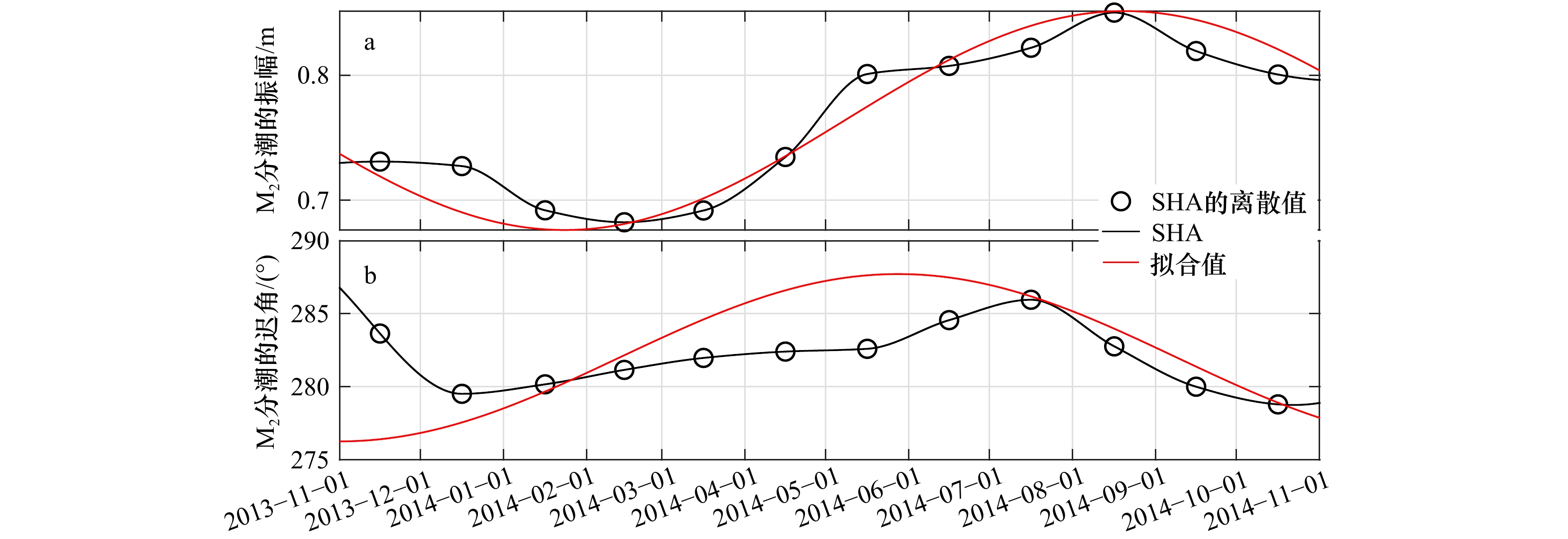
    在人造“水位数据”中,假设M2分潮的振幅和迟角是随时间变化的,而其他信号的振幅和迟角均是常数。另外,MK3、M4、LF1和LF2被视为噪声,不估计其振幅和迟角。为了获得M2分潮振幅和迟角较为真实的时间变化,在不考虑节点调制的情况下,通过SHA分析了E2的真实水位数据,如图4所示。结果表明,M2分潮的振幅和迟角存在明显的时间变化。为了获得更加平滑的时间变化特征,利用正弦函数对SHA方法所得M2分潮振幅和迟角进行了拟合。图4中的红线展示了拟合结果,拟合公式如下:

    图  4  使用SHA分析E2站水位观测数据所获得M2分潮时变的振幅(a)和迟角(b)及其拟合值
    Figure  4.  The temporally varying amplitude (a) and phase lag (b) of the M2 constituent obtained by analyzing the observed sea level at E2 Station using SHA and their fitting values
    $$a_{{{\rm{M}}_2}}^{'}(t){\rm{ = }}0.087\;5 \sin \left( {0.015\;1 t - 1.137\;7} \right) + 0.763\;8,$$ (6)
    $$\varphi _{{{\rm{M}}_2}}^{'}(t){\rm{ = }}5.784\;9 \sin \left( {0.015\;1 t - 35.088\;3} \right) + 281.989\;3,$$ (7)

    式中,t表示从世界时0年1月0日起经过的时间(即MATLAB中的“datenum”值),单位:d;此外,t的范围为2013年11月1日至2014年11月1日,与E2站实际水位观测数据的时间范围相同;$a_{{{\rm{M}}_2}}^{'}$是M2分潮的时变振幅,单位:m;$\varphi _{{{\rm{M}}_2}}^{'}$为M2分潮的时变迟角,单位:(°)。参考CHA[9],由M2分潮引起的水位变化的表达式为下

    $${\zeta _{{{\rm{M}}_2}}} = a_{{{\rm{M}}_2}}^{'}(t) \cdot \cos \left[ {{\omega _{{{\rm{M}}_2}}} \cdot (t - {t_{{\rm{mid}}}}) - \varphi _{{{\rm{M}}_2}}^{'}(t) \cdot {\text π} /180} \right],$$ (8)

    式中,tmidt的中值。

    为了获得其他潮汐信号较为真实的振幅和迟角,在不考虑节点调制的情况下,使用CHA分析了E2处的海平面数据,得到的常数形式的振幅和迟角如表1所示。LF1和LF2的迟角设置为4个主要分潮的平均迟角,并根据功率谱密度的结果,通过反复试验得到了振幅值,见表1。由上述信号引起的水位变化与M2分潮引起的水位变化具有类似的形式(即式(8)),此处不再赘述。

    表  1  理想实验中的潮汐成分及其常数形式的振幅和迟角
    Table  1.  The prescribed constant amplitudes and phase lags of the constituents in ideal twin experiments
    分潮给定值
    振幅/cm迟角/(°)
    S220.69273.88
    K127.1975.46
    O120.4514.70
    MK30.83314.20
    M41.02246.79
    LF16.00161.73
    LF24.00161.73
    下载: 导出CSV 
    | 显示表格

    从人造“水位数据”的功率谱密度(图3)可以看出,人造“水位数据”成功地再现了E2站M2、S2、K1、O1、MK3、M4、LF1、LF2等信号,且不包含其他频段的信号,表明由已知的振幅和迟角构造的“水位数据”可以作为E2站真实水位观测数据的替代品。

    2.3.2   实验和结果

    在理想实验中,不考虑节点调制,采用CHA、SHA、OEHA和EHA分析人造“水位数据”,以获得M2、S2、K1和O1 4个主要分潮的振幅和迟角,除此之外,人造“水位数据”中的其他信号,被视作噪声[20]。在使用SHA时,每个月的数据作为一段进行分析,根据瑞利准则,区分上述4个主要分潮的最小周期为14.8 d[21],因此,只有当该段数据长度大于15 d时,SHA才对该段数据进行分析。此外,采用3次样条插值法对每段所得离散的振幅和迟角进行插值以获得连续的结果。Pan等[14]指出,在不同独立点数下,EHA得到的时变振幅和迟角代表了不同时间尺度上的变化。根据Jin等[10]的研究结果,在下面的理想实验中,OEHA和EHA的独立点数被设为5,比季节数(春、夏、秋、冬)多1。

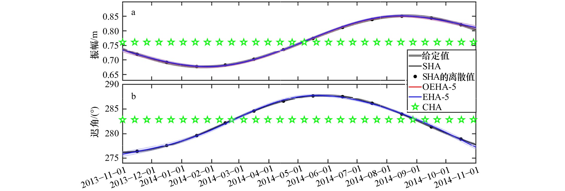
    图5所示,SHA、OEHA和EHA得到的M2分潮时变的振幅和迟角几乎等于给定值;CHA得到的结果是恒定的,不能捕捉到M2分潮的时间变化,而SHA、OEHA和EHA可以得到M2分潮的时间变化特征。

    图  5  理想实验中给定的M2分潮振幅(a)和迟角(b),以及使用SHA、采用5个独立点的OEHA、采用5个独立点的EHA和CHA得到的结果
    Figure  5.  The amplitude (a) and phase lag (b) of the M2 constituent prescribed in ideal experiments and the estimated values using SHA, OEHA with 5 independent points, EHA with 5 independent points, and CHA

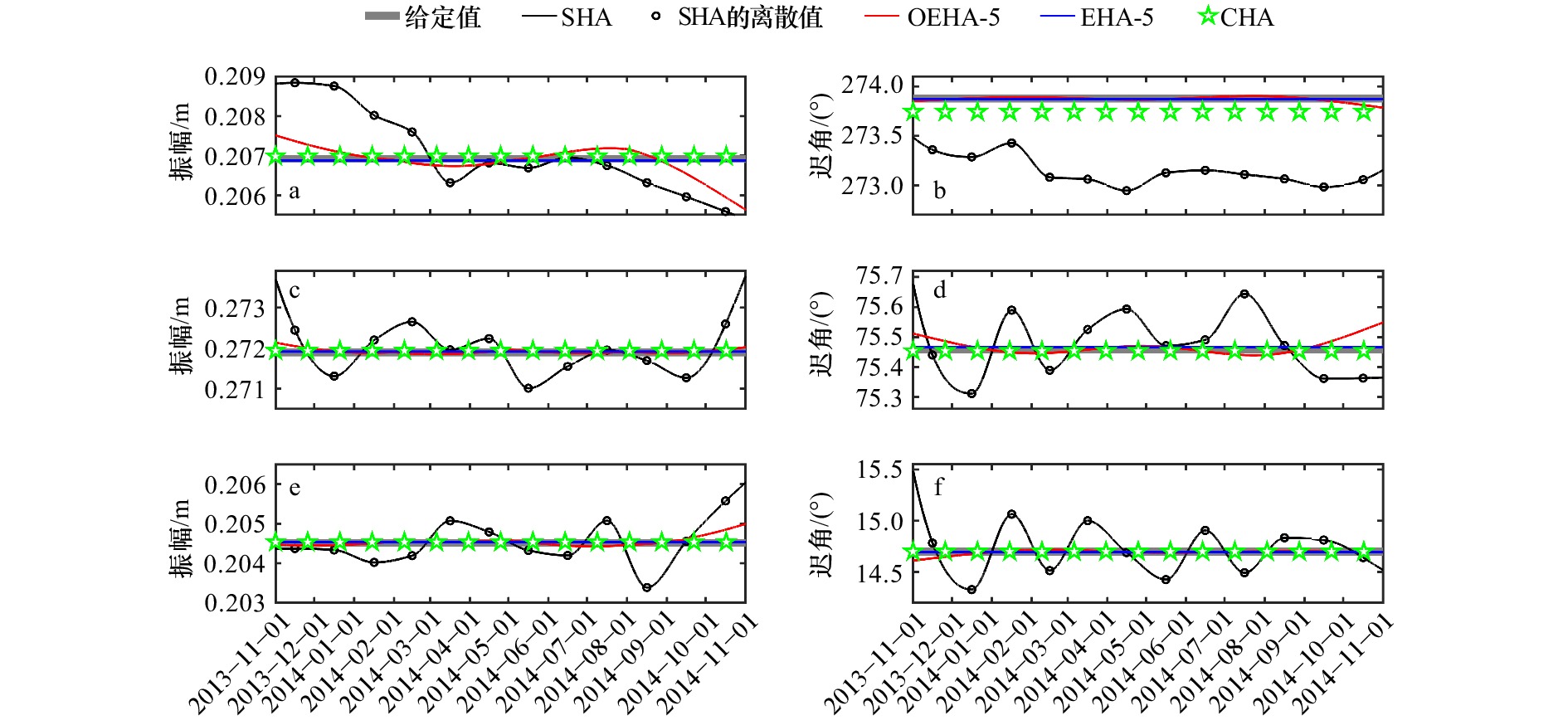
    对于S2分潮而言,EHA分析所得振幅和迟角比CHA所得结果更接近给定值(图6a图6b),而SHA的结果与给定值相差甚远,尤其是迟角(图6b),这主要是因为M2分潮和S2分潮的频率很接近,当同时被假定为随时间变化时,分析结果可能会互相影响。使用OEHA时,除2014年10月和11月外,S2分潮的迟角几乎都等于给定值;此外,得到的S2分潮的振幅是时变的,与给定值有一定的偏差。对于K1分潮(图6c图6d)和O1分潮(图6e图6f),CHA和EHA所得结果几乎等于给定值,而OEHA得到的振幅和迟角整体上接近给定值,但在端点处差距较大,SHA分析所得振幅和迟角具有明显的时间变化特征,与给定值相差较大。总的来说,虽然SHA、OEHA和EHA均能成功估计M2分潮的时间变化特征,但EHA所得其他3个主要分潮的振幅和迟角与给定值吻合最好。

    图  6  理想实验中给定的S2分潮(a,b)、K1分潮(c,d)和O1分潮(e,f)的振幅和迟角,以及使用SHA、采用5个独立点的OEHA、采用5个独立点的EHA和CHA得到的结果
    Figure  6.  The amplitude and phase lag of the S2 (a, b), K1 (c, d) and O1 (e, f) constituent prescribed in ideal experiments and the estimated values using SHA, OEHA with 5 independent points, EHA with 5 independent points, and CHA

    需要注意的是,E1站的实际水位观测数据存在部分缺测,这可能会对分析结果造成影响。在理想敏感实验中,根据E1站的缺测时段,剔除了人造“水位数据”中相应的数据,进而利用CHA、SHA、OEHA、EHA对其进行了分析。虽然大约1/4的时段没有“水位数据”,但是OEHA和EHA所得结果很好地捕获了M2分潮给定振幅和迟角的时间变化特征(图7a图7b)。相反,SHA所得M2分潮的振幅和迟角与给定值略有偏差,特别是在2013年11月至2014年2月期间,这主要是因为2013年12月和2014年1月的缺测较多,导致这两个月的“水位数据”没有被分析而无法获得M2分潮振幅和迟角值。EHA分析得到的M2分潮所引起的水位变化与给定的M2分潮所导致的水位变化之间的绝均差为0.19 cm;而SHA所得绝均差为0.28 cm,约为没有缺测时的4.5倍。对于S2、K1和O1分潮,CHA分析所得振幅和迟角值与给定值之间的差距比理想实验中的差距更大,如图8所示;此外,“水位数据”的缺测对SHA和OEHA的结果也有很大的影响,OEHA分析所得3个分潮的振幅和迟角与给定值之间的误差变得更大。相反,EHA得到的S2和K1分潮的振幅和迟角仍然接近给定值。虽然EHA对O1分潮的分析结果与给定值略有偏差,但差异明显小于CHA、SHA和OEHA的结果。由此可见,EHA总体上优于CHA、SHA和OEHA。

    图  7  理想敏感实验中给定的M2分潮振幅(a)和迟角(b),以及使用SHA、采用5个独立点的OEHA、采用5个独立点的EHA和CHA得到的结果
    b中的洋红色实线描述了理想敏感实验中人造“水位数据”的时间段
    Figure  7.  The amplitude (a) and phase lag (b) of the M2 constituent prescribed in ideal sensitivity experiments and the estimated values using SHA, OEHA with 5 independent points, EHA with 5 independent points, and CHA
    The magenta solid line in b describes the temporal locations of the artificial sea level observations in the ideal sensitivity experiment
    图  8  理想敏感实验中给定的S2分潮(a, b)、K1分潮(c, d)和O1分潮(e, f)的振幅和迟角,以及使用SHA、采用5个独立点的OEHA、采用5个独立点的EHA和CHA得到的结果
    每个子图中的洋红色实线描述了理想敏感实验中人造“水位数据”的时间段
    Figure  8.  The amplitude and phase lag of the S2 (a, b), K1 (c, d) and O1 (e, f) constituent prescribed in ideal sensitivity experiments and the estimated values using SHA, OEHA with 5 independent points, EHA with 5 independent points, and CHA
    The magenta solid lines in each panels describe the temporal locations of the artificial sea level observations in the ideal sensitivity experiment

    总体而言,无论“水位数据”中是否存在缺测,在利用EHA进行分析时,M2分潮时变振幅和迟角以及其他分潮调和常数的给定值都能被准确反演,说明EHA能有效分离具有不同变化特征的潮汐信号,可用于实际实验中M2分潮的季节变化研究。

    为了确定基准实验中所需分析的潮汐成分,利用CHA对E1和E2站的水位观测数据进行了调和分析,根据信噪比的大小[9, 22]选择了M2、K1、S2和O1 4个最重要的成分作为进行分析的分潮。利用EHA进行数据分析时,独立点数设置为5,仅将M2分潮的振幅和迟角假定为随时间变化。

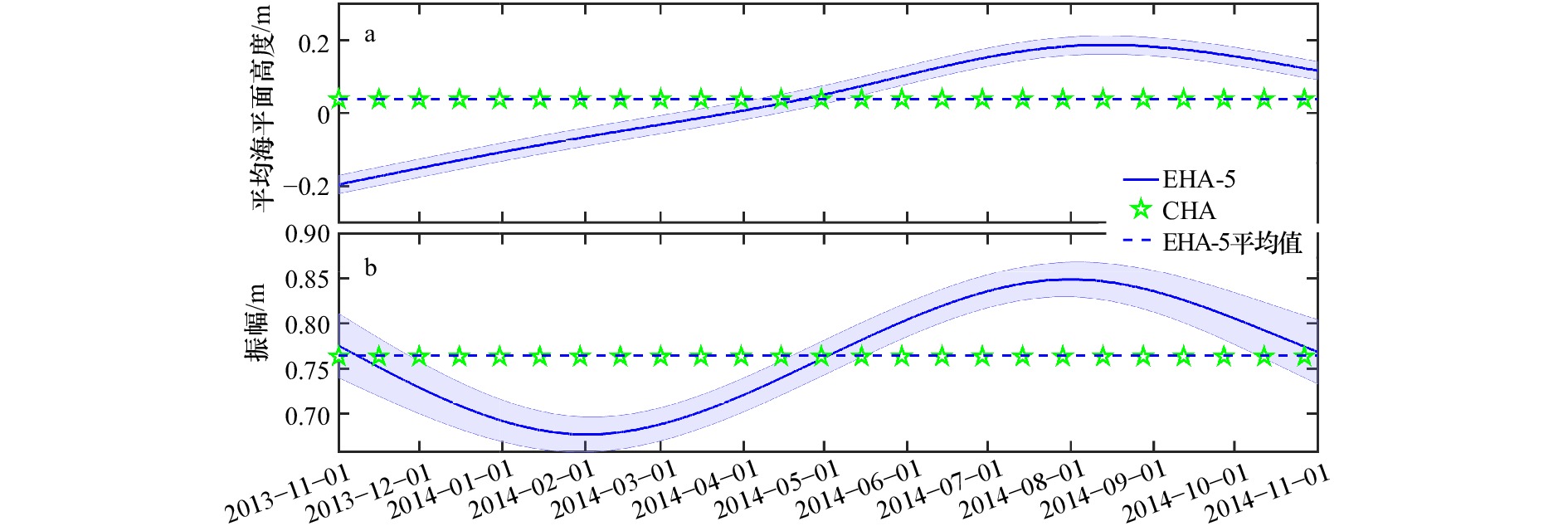
    CHA和EHA所得E2站M2分潮振幅的分析结果如图9b所示。从图中可以看出,EHA分析所得M2分潮振幅具有明显的季节变化特征,其平均值与CHA分析所得常数形式的M2分潮振幅几乎相等,说明了EHA所得分析结果的合理性。

    图  9  E2站基准实验的实验结果
    蓝色实线展示了采用5个独立点的EHA得到的平均海平面高度(a)和M2分潮振幅(b)的时变值,蓝色虚线为采用5个独立点的EHA得到的平均海平面高度(a)和M2分潮振幅(b)的平均值,绿色星号表示常数形式的平均海平面高度(a)和M2分潮振幅(b),蓝色阴影表示相应的95%置信区间
    Figure  9.  The results of benchmark experiment at E2 Station
    The blue solid line shows the time-varying values of mean sea level (a) and M2 constituent amplitude (b) obtained by EHA at 5 independent points, the blue dotted line shows the average value of mean sea level (a) and M2 constituent amplitude (b) obtained by EHA at 5 independent points, and the green stars describe the constant mean sea level (a) and M2 constituent amplitude (b), the blue shadings indicate the corresponding 95% confidence intervals

    EHA所得随时间变化的M2振幅在夏季(大约7−8月)达到最大值,在冬季(大约1−2月)达到最小值,夏季M2分潮振幅比年平均值大8.42 cm(约11.01%),而冬季值比年平均值小8.76 cm(约11.46%),其季节变化幅度远大于在观测期内由18.6 a的节点调制引起的振幅变化(不超过1%)。表2列出了CHA和EHA在E2站分析所得其他分潮的振幅值,可以看出,EHA和CHA分析所得其他3个主要分潮的常数形式的振幅值之间的绝均差最大仅为0.07 cm,进一步表明EHA不仅可以准确提取M2分潮振幅的季节变化特征,也能准确得到其他分潮的常数形式的振幅。

    表  2  基准实验中CHA和EHA分析所得4个主要分潮的振幅(单位:cm)
    Table  2.  The amplitudes of four main tidal constituents obtained by CHA and EHA in the benchmark experiment (unit: cm)
    站点分潮CHAEHA
    E1M2103.53102.96
    K129.0429.14
    S229.4929.50
    O122.8922.90
    E2M276.3376.46
    K127.1927.21
    S220.6920.62
    O120.4520.44
      注:由于M2分潮的振幅是假定随时间变化的,因此使用EHA时列出其平均值。
    下载: 导出CSV 
    | 显示表格

    CHA和EHA分析所得E2站MSL如图9a所示。可以看出,EHA分析所得随时间变化的MSL的平均值几乎等于CHA分析所得常数形式的MSL,进一步表明EHA的结果是合理的。但是需要注意的是,EHA分析所得E2站处MSL在1年内的变化约为0.4 m,远大于传统上MSL的全球平均变化(约为0.001 m/a)[23-24],这主要是因为EHA中随时间变化的MSL包含气象因素导致的水位变化(式(3))。如Lü等[18]所述,风速和气压等气象因素均会影响到低频水位的变化,因此包含了气象因素影响的MSL在2013年11月和2014年11月存在一定的差异,该现象在E1站同样存在。EHA分析所得时变MSL的最大值出现在夏季,而最小值出现在冬季。与M2分潮振幅的时间变化特征相似,EHA分析所得MSL的时间变化比较平稳,且不存在季节变化之外的信号。

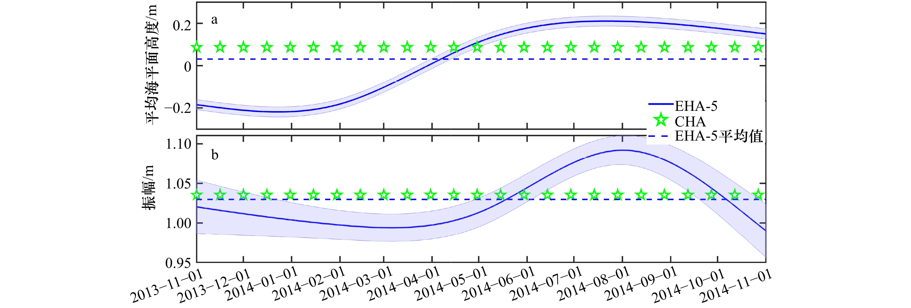
    CHA和EHA分析所得E1站MSL和M2分潮振幅的结果如图10所示。可以看出,EHA分析所得随时间变化的M2分潮振幅比较平滑,且与E2站具有相同的变化趋势。在夏季,M2分潮振幅增加了约6.05%,而在冬季则减少了3.85%,这比在观测期内由18.6 a节点调制引起的不超过1%的振幅变化大得多。从表2中可以看出,EHA分析所得其他3个分潮的常数形式的振幅与CHA分析所得结果非常接近。此外,EHA分析所得随时间变化的MSL在夏季达到最大值,在冬季达到最小值,与E1站M2分潮的季节变化特征相同。需要注意的是,E1站和E2站相距较近,但对比图9a图10a发现,E1站和E2站的平均海平面的年变化并不完全一致,E2站MSL的最小值出现在11月,而E1站MSL的最小值出现在1月,这是由于E1站2014年1月和2月的数据存在缺测,会给该时间段的平均海平面的计算带来偏差,从而影响最小MSL出现的月份,但并没有显著影响两站的M2分潮振幅和MSL的变化趋势,表明EHA在即使存在缺测的E1站,也可以得到相对合理的结果。

    图  10  E1站基准实验的实验结果
    蓝色实线展示了采用5个独立点的EHA得到的平均海平面高度(a)和M2分潮振幅(b)的时变值,蓝色虚线为采用5个独立点的EHA得到的平均海平面高度(a)和M2分潮振幅(b)的平均值,绿色星号表示常数形式的平均海平面高度(a)和M2分潮振幅(b),蓝色阴影表示相应的95%置信区间
    Figure  10.  The results of benchmark experiment at E1 Station
    The blue solid line shows the time-varying values of mean sea level (a) and M2 constituent amplitude (b) obtained by EHA at 5 independent points, the blue dotted line shows the average value of mean sea level (a) and M2 constituent amplitude (b) obtained by EHA at 5 independent points, and the green stars describe the constant mean sea level (a) and M2 constituent amplitude (b), the blue shadings indicate the corresponding 95% confidence intervals

    综上所述,EHA在E1站和E2站分析所得M2分潮振幅具有相同的季节变化特征:夏季大,冬季小。E2站M2分潮振幅的相对变化约为11%,在E1站约为5%,这与Foreman等[11]、Huess和Andersen[4]的结果(6%),以及Müller等[2]根据模型和观测数据所分析的结果(5%~10%)相近。此外,EHA在E1站和E2站分析所得时变MSL具有与M2分潮振幅相同的季节性变化,这表明MSL可能是导致M2分潮振幅季节变化的因素之一,因为潮波的传播受到水深的影响[13]

    在基准实验中,选择了4个主要分潮进行评估,并且假定只有M2分潮的振幅和迟角随时间变化。当其他分潮也被分析或其他分潮振幅和迟角也被假定为随时间变化时,M2分潮的分析结果可能会受到影响。因此,对E2站的数据进行了一些新的实验来测试EHA分析所得的M2分潮振幅季节变化特征对分潮选择的敏感性。如表3所示,在敏感性实验SE11−SE13中,对M2,K1,S2和O1 4个分潮进行分析,这与基准实验相同,但具有时变振幅和迟角的分潮不同;在敏感性实验SE21−SE24中,与基准实验不同的是,将对M2、K1、S2、O1、N2、K2、P1和Q1 8个分潮进行分析,且振幅和迟角随时间变化的分潮也发生了变化。

    表  3  实际实验中的详细实验设置
    Table  3.  The detailed experimental settings of the practical experiments
    实验名分析的分潮具有时变特征的分潮有无缺测
    基准实验M2, K1, S2, O1M2
    SE11M2, K1, S2, O1M2, K1
    SE12M2, K1, S2, O1M2, K1, S2
    SE13M2, K1, S2, O1M2, K1, S2, O1
    SE21M2, K1, S2, O1, N2, K2, P1, Q1M2
    SE22M2, K1, S2, O1, N2, K2, P1, Q1M2, K1
    SE23M2, K1, S2, O1, N2, K2, P1, Q1M2, K1, S2
    SE24M2, K1, S2, O1, N2, K2, P1, Q1M2, K1, S2, O1
    SE31M2, K1, S2, O1M2有(同E1)
    SE32−SE35M2, K1, S2, O1M2有(大约占1/4)
    下载: 导出CSV 
    | 显示表格

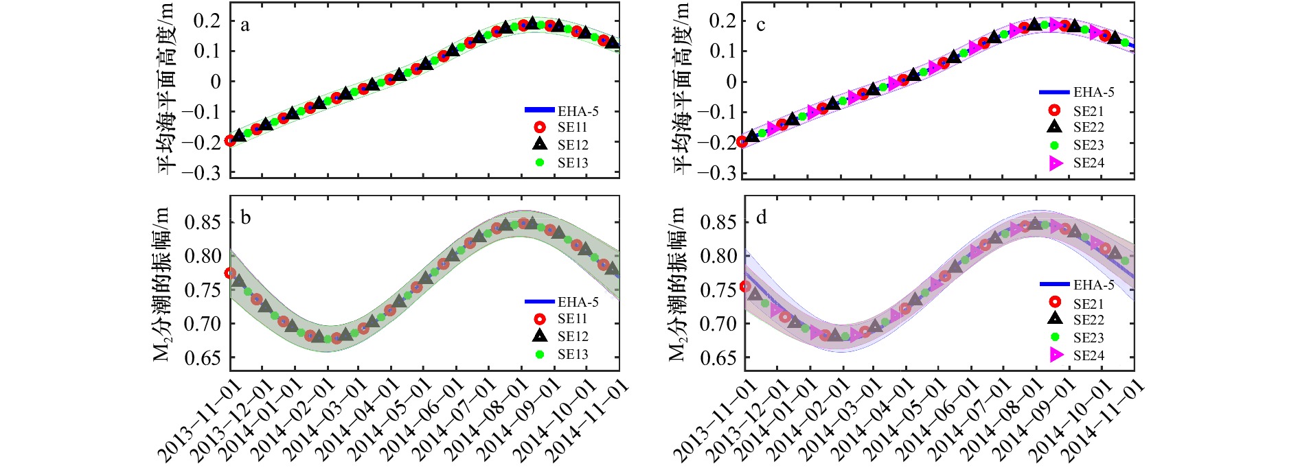
    上述敏感性实验中,EHA分析所得随时间变化的MSL和M2分潮振幅如图11所示。可以看出,当具有时变特征的分潮发生改变时(SE11−SE13),EHA分析所得随时间变化的M2分潮振幅和MSL几乎与基准实验的结果完全一致。当分析的分潮数目发生变化时(SE21−SE24),EHA分析所得随时间变化的MSL与基准实验的结果几乎完全一致(图11c);此外,虽然随时间变化的M2分潮振幅与基准实验结果不完全相同,但整体变化趋势是一致的(图11d)。值得注意的是,SE21−SE24中随时间变化的M2分潮振幅几乎彼此相等,这与SE11−SE13所得结论一致。上述结果表明,EHA中被分析的分潮和具有时变特征的分潮的选取并不会影响分析所得M2分潮振幅和MSL的时间变化趋势和季节变化特征。

    图  11  分潮选择的敏感性实验结果
    蓝色实线表示采用5个独立点的EHA在基准实验中的结果。带颜色的阴影表示相应的95%置信区间
    Figure  11.  The results on the sensitivity of tidal constituent selection
    The blue solid line represents the results of EHA with 5 independent points in the benchmark experiment. The shadings with colors indicate the corresponding 95% confidence intervals

    时变M2分潮振幅和MSL的分析结果也可能会受到数据缺测的影响。因此,利用E2站的数据进行了一系列实验以测试EHA分析结果对数据缺测的敏感性。如表3所示,在敏感性实验SE31中,根据E1点缺测情况,相应地剔除了E2站水位观测数据。E1站水位数据中存在大约1/4的缺测,因此,为了进一步检验数据缺失的影响,将E2站水位观测数据平均分为4份,并将这4份水位观测数据分别作为SE32−SE35中的缺测数据。其他实验设置与基准实验完全相同。

    敏感性实验SE31−SE35的结果如图12所示。可以看出,由于SE31−SE35的水位观测数据存在约1/4的数据缺失,因此EHA分析所得M2分潮振幅和MSL均与基准实验中的值不完全相同。对比实验SE31和基准实验中分析所得E2站MSL的结果,可以看到当E2站数据在2014年1月和2014年2月出现缺测时,虽然MSL的最小值出现的月份在2013年11月,但是这种现象并没有数据无缺测时那么显著,并且2013年11月至2014年2月的分析结果与无缺测时的分析结果存在明显的差异,说明了数据缺失是导致E1站和E2站MSL最小值出现月份不同的原因。但是,SE31−SE35中所得M2分潮振幅和MSL的变化趋势与基准实验中的相同:夏季大,冬季小。实验结果表明,数据在某一月份的集中缺测会给该月的计算结果带来影响,但不会显著影响EHA分析所得M2分潮振幅和MSL的季节变化特征,并进一步论证了EHA所得E1站的M2分潮振幅季节变化是合理、可信的。

    图  12  数据缺失和独立点数的敏感性实验结果
    蓝色实线表示采用5个独立点的EHA在基准实验的结果。带颜色的阴影表示相应的95%置信区间
    Figure  12.  The results on the sensitivity of missing data and independent points
    The blue solid line indicates the results of EHA with 5 independent points in the benchmark experiment. The shadings with colors indicate the corresponding 95% confidence intervals

    Jin等[10]指出,如何选择EHA中的独立点是一个需要进一步研究的问题。而Pan等[14]则指出,EHA在不同独立点数时所得到的分析结果代表了不同时间尺度上的振荡。同样地,选择合适的独立点数对EHA的表现也非常重要,尤其是对于E1站非连续的水位数据。因此在新的敏感性实验中尝试了4个、6个、7个和8个等不同的独立点数。

    图12d所示,当独立点数取为季节数的两倍(即:8)时,EHA分析所得E2站的M2分潮振幅的时间变化趋势与基准实验结果一致,但存在除季节变化之外的震荡,结果表明:EHA中,独立点越多并不一定会得到更真实的结果。

    当独立点数大于3且小于8时,EHA分析所得M2振幅和MSL的结果并不完全与5个独立点时的结果等同,但其季节性变化趋势相同。如Pan等[14]所述,不同独立点数得到的结果不同,可能是因为采用不同独立点数的EHA得到的结果包含了不同的信号。以上所有敏感性实验的结果表明:EHA分析所得E2站M2分潮振幅的季节变化特征是鲁棒的,不受实验设置的影响。

    平均海平面、层化和涡动黏性系数的季节变化是造成沿海地区M2分潮振幅呈现季节性变化的主要原因[4, 13, 15]。渤海湾的风场不仅对平均海平面有重大影响[18],因受东亚季风影响而具有明显的季节变化特征[25]。此外,季风还可以影响层化涡动黏性系数[26-29]。参照Devlin等[1],采用北太平洋季风指数(WNPMI)来表征东亚季风[30]。WNPMI下载网址为:http://apdrc.soest.hawaii.edu/projects/monsoon/daily-data.html#mon。如图13所示,WNPMI与E1站和E2站M2分潮振幅具有显著的正相关,相关系数分别为0.86和0.87,表明:东亚季风可能是造成渤海湾M2分潮振幅季节性变化的内在原因。

    图  13  北太平洋季风指数(WNPMI)与E1站和E2站M2分潮振幅的相关性
    黑点表示每天的WNPMI,黑圈表示WNPMI的月平均值,黑线为使用三次样条插值法对WNPMI的月平均值进行拟合的结果,蓝线为采用5个独立点的EHA得到的M2分潮振幅,黑色竖线和蓝色阴影表示相应的95%置信区间
    Figure  13.  The correlation between WNPMI and M2 constituent amplitude of E1 and E2 stations
    The black dot represents the daily WNPMI, the black circle represents the monthly average value of WNPMI, the black line is the result of fitting the monthly average value of WNPMI using cubic spline interpolation method, and the blue line is the M2 constituent amplitude obtained by EHA with 5 independent points, the black vertical bars and the blue shadings indicate the corresponding 95% confidence intervals

    根据前人研究结果,我们大胆猜测,东亚季风可能通过以下3个途径来影响渤海湾M2分潮振幅的季节变化:

    (1)影响平均海平面的季节变化。亚洲季风导致了径流的季节性变化[31],使得超过60%的黄河水在夏季入海[32],也使得海河夏季的入海量是冬季的两倍左右[33];与此同时,夏季东亚季风导致的渤海上空的东南风使一部分黄河水向北输送到渤海湾[28],加上直接汇入渤海湾的海河入海量也增大,使得夏季渤海湾的淡水汇入增多[34]。另一方面,受东亚季风影响,夏季通过渤海海峡从渤海进入黄海的通量比冬季更小[27]。综上,受东亚季风影响,夏季从黄河和海河汇入渤海湾的淡水增加,与此同时,从渤海流出到黄海的海水更少,共同导致夏季渤海湾平均海平面更高。而潮波的传播受到水位的影响[13],因此,受东亚季风季节变化影响的渤海湾平均海平面的季节变化导致了M2分潮振幅的季节变化。

    (2)影响层化的季节变化。根据Yanagi等[35]和Jeon等[26]的研究,对于渤海湾而言,冬季从陆地到海洋的强西北风会导致海水降温,破坏之前形成的层化并导致垂向均一的层化状态。春末夏初,随着海水表层升温速率的增加以及黄河和海河入海量的增加,海面风应力和底部摩擦力引起的混合不足以消耗输入的势能,使得渤海湾层化逐渐加强[36-37],并在夏季达到最大值[37]。因此,东亚季风能够导致层化的季节变化,进而引起M2分潮的季节变化[2]

    (3)影响涡动黏性系数。Pohlmann[38]发现北海的垂向涡黏性具有显著的年周期并与海面风应力的年变化有关;此外,垂直涡动黏性系数依赖于层化。Maas和Van Haren[39]证实了层化情况下涡动黏性系数降低的可能性。Howarth[40]认为温跃层的存在可以降低涡动黏性系数,除此之外,Müller等[2]指出,层化可以使得水体更加稳定,进而导致夏季的涡动黏性系数比混合均匀的夏季小几个数量级。因此,受东亚季风影响的层结的季节变化会导致涡动黏性系数的季节变化,进而诱发M2分潮的季节变化。

    除了东亚季风可能影响渤海湾M2振幅的季节变化之外,水深、近岸与否等原因也有可能会对M2分潮振幅的季节变化造成影响。对比图9图10可知,E1站和E2站的MSL和M2分潮振幅的年变化并不完全一致,这种现象一方面是由数据缺测造成的,另一方面也可能与E1和E2两站的水深、近岸与否的差异有关。Müller等[2]认为,相比远离海岸的地区,近岸地区的M2分潮的季节变化更显著。而在渤海地区,不同的水深和底摩擦系数也会对M2分潮的振幅带来影响[42]

    本文利用EHA分析了渤海湾E1站和E2站一年时间段的水位观测数据,同时估计了时变的和不随时间变化的分潮振幅和迟角,来探究渤海湾M2分潮振幅的季节变化。

    在理想实验中,根据E2站的水位观测数据构建了人造“水位数据”,其中,M2分潮具有时变的振幅和迟角,而S2、K1、O1、MK3、M4分潮及LF1和LF2的振幅或迟角是常数。实验结果表明:无论人造“水位数据”是否存在缺测,EHA分析所得随时间变化的M2振幅和迟角以及不随时间变化的S2、K1和O1分潮的振幅和迟角整体比CHA、SHA、OEHA等方法的分析结果更接近给定值,表明EHA是一种行之有效的方法。

    利用EHA分析实际水位观测数据时,分析结果发现,E1站和E2站时变M2分潮振幅具有相同的变化趋势:夏季大、冬季小。此外,M2分潮振幅的相对变化在E2站约为11%,在E1站约为5%。E1站和E2站随时间变化的平均海平面与M2分潮振幅随时间变化的趋势相同。EHA分析所得其他潮汐成分(包括S2,K1和O1)的常数形式的振幅值与CHA所得结果吻合较好。更重要的是,敏感实验的结果表明,M2分潮振幅和平均海平面的变化趋势是鲁棒的,不受实验设置的影响。根据前人研究[2-3, 11, 13, 41]猜测,东亚季风的季节变化引起了平均海平面、层化和涡动黏性系数的季节变化,进而诱导了渤海湾M2分潮振幅的季节变化。

  • 图  1  渤海湾观测站E1和E2的位置(红星),以及10 m和40 m水深线

    Fig.  1  The locations of the observation stations (E1 and E2, red stars) in the Bohai Bay, and the isobathymetric lines at 10 m and 40 m

    图  2  E1(a)和E2(b)站的水位观测数据

    洋红色实线描述了观测的时间段

    Fig.  2  The observed sea level at E1(a) and E2(b) stations

    The magenta solid lines describe the temporal locations of the observations

    图  3  E2站水位数据和人造“水位数据”的功率谱密度

    黑色和红色虚线表示相应的95%置信值

    Fig.  3  The power spectral densities of the observed sea level at E2 Station and the artificial sea level

    The black and red dashed lines designate the corresponding 95% significance level against red noise

    图  4  使用SHA分析E2站水位观测数据所获得M2分潮时变的振幅(a)和迟角(b)及其拟合值

    Fig.  4  The temporally varying amplitude (a) and phase lag (b) of the M2 constituent obtained by analyzing the observed sea level at E2 Station using SHA and their fitting values

    图  5  理想实验中给定的M2分潮振幅(a)和迟角(b),以及使用SHA、采用5个独立点的OEHA、采用5个独立点的EHA和CHA得到的结果

    Fig.  5  The amplitude (a) and phase lag (b) of the M2 constituent prescribed in ideal experiments and the estimated values using SHA, OEHA with 5 independent points, EHA with 5 independent points, and CHA

    图  6  理想实验中给定的S2分潮(a,b)、K1分潮(c,d)和O1分潮(e,f)的振幅和迟角,以及使用SHA、采用5个独立点的OEHA、采用5个独立点的EHA和CHA得到的结果

    Fig.  6  The amplitude and phase lag of the S2 (a, b), K1 (c, d) and O1 (e, f) constituent prescribed in ideal experiments and the estimated values using SHA, OEHA with 5 independent points, EHA with 5 independent points, and CHA

    图  7  理想敏感实验中给定的M2分潮振幅(a)和迟角(b),以及使用SHA、采用5个独立点的OEHA、采用5个独立点的EHA和CHA得到的结果

    b中的洋红色实线描述了理想敏感实验中人造“水位数据”的时间段

    Fig.  7  The amplitude (a) and phase lag (b) of the M2 constituent prescribed in ideal sensitivity experiments and the estimated values using SHA, OEHA with 5 independent points, EHA with 5 independent points, and CHA

    The magenta solid line in b describes the temporal locations of the artificial sea level observations in the ideal sensitivity experiment

    图  8  理想敏感实验中给定的S2分潮(a, b)、K1分潮(c, d)和O1分潮(e, f)的振幅和迟角,以及使用SHA、采用5个独立点的OEHA、采用5个独立点的EHA和CHA得到的结果

    每个子图中的洋红色实线描述了理想敏感实验中人造“水位数据”的时间段

    Fig.  8  The amplitude and phase lag of the S2 (a, b), K1 (c, d) and O1 (e, f) constituent prescribed in ideal sensitivity experiments and the estimated values using SHA, OEHA with 5 independent points, EHA with 5 independent points, and CHA

    The magenta solid lines in each panels describe the temporal locations of the artificial sea level observations in the ideal sensitivity experiment

    图  9  E2站基准实验的实验结果

    蓝色实线展示了采用5个独立点的EHA得到的平均海平面高度(a)和M2分潮振幅(b)的时变值,蓝色虚线为采用5个独立点的EHA得到的平均海平面高度(a)和M2分潮振幅(b)的平均值,绿色星号表示常数形式的平均海平面高度(a)和M2分潮振幅(b),蓝色阴影表示相应的95%置信区间

    Fig.  9  The results of benchmark experiment at E2 Station

    The blue solid line shows the time-varying values of mean sea level (a) and M2 constituent amplitude (b) obtained by EHA at 5 independent points, the blue dotted line shows the average value of mean sea level (a) and M2 constituent amplitude (b) obtained by EHA at 5 independent points, and the green stars describe the constant mean sea level (a) and M2 constituent amplitude (b), the blue shadings indicate the corresponding 95% confidence intervals

    图  10  E1站基准实验的实验结果

    蓝色实线展示了采用5个独立点的EHA得到的平均海平面高度(a)和M2分潮振幅(b)的时变值,蓝色虚线为采用5个独立点的EHA得到的平均海平面高度(a)和M2分潮振幅(b)的平均值,绿色星号表示常数形式的平均海平面高度(a)和M2分潮振幅(b),蓝色阴影表示相应的95%置信区间

    Fig.  10  The results of benchmark experiment at E1 Station

    The blue solid line shows the time-varying values of mean sea level (a) and M2 constituent amplitude (b) obtained by EHA at 5 independent points, the blue dotted line shows the average value of mean sea level (a) and M2 constituent amplitude (b) obtained by EHA at 5 independent points, and the green stars describe the constant mean sea level (a) and M2 constituent amplitude (b), the blue shadings indicate the corresponding 95% confidence intervals

    图  11  分潮选择的敏感性实验结果

    蓝色实线表示采用5个独立点的EHA在基准实验中的结果。带颜色的阴影表示相应的95%置信区间

    Fig.  11  The results on the sensitivity of tidal constituent selection

    The blue solid line represents the results of EHA with 5 independent points in the benchmark experiment. The shadings with colors indicate the corresponding 95% confidence intervals

    图  12  数据缺失和独立点数的敏感性实验结果

    蓝色实线表示采用5个独立点的EHA在基准实验的结果。带颜色的阴影表示相应的95%置信区间

    Fig.  12  The results on the sensitivity of missing data and independent points

    The blue solid line indicates the results of EHA with 5 independent points in the benchmark experiment. The shadings with colors indicate the corresponding 95% confidence intervals

    图  13  北太平洋季风指数(WNPMI)与E1站和E2站M2分潮振幅的相关性

    黑点表示每天的WNPMI,黑圈表示WNPMI的月平均值,黑线为使用三次样条插值法对WNPMI的月平均值进行拟合的结果,蓝线为采用5个独立点的EHA得到的M2分潮振幅,黑色竖线和蓝色阴影表示相应的95%置信区间

    Fig.  13  The correlation between WNPMI and M2 constituent amplitude of E1 and E2 stations

    The black dot represents the daily WNPMI, the black circle represents the monthly average value of WNPMI, the black line is the result of fitting the monthly average value of WNPMI using cubic spline interpolation method, and the blue line is the M2 constituent amplitude obtained by EHA with 5 independent points, the black vertical bars and the blue shadings indicate the corresponding 95% confidence intervals

    表  1  理想实验中的潮汐成分及其常数形式的振幅和迟角

    Tab.  1  The prescribed constant amplitudes and phase lags of the constituents in ideal twin experiments

    分潮给定值
    振幅/cm迟角/(°)
    S220.69273.88
    K127.1975.46
    O120.4514.70
    MK30.83314.20
    M41.02246.79
    LF16.00161.73
    LF24.00161.73
    下载: 导出CSV

    表  2  基准实验中CHA和EHA分析所得4个主要分潮的振幅(单位:cm)

    Tab.  2  The amplitudes of four main tidal constituents obtained by CHA and EHA in the benchmark experiment (unit: cm)

    站点分潮CHAEHA
    E1M2103.53102.96
    K129.0429.14
    S229.4929.50
    O122.8922.90
    E2M276.3376.46
    K127.1927.21
    S220.6920.62
    O120.4520.44
      注:由于M2分潮的振幅是假定随时间变化的,因此使用EHA时列出其平均值。
    下载: 导出CSV

    表  3  实际实验中的详细实验设置

    Tab.  3  The detailed experimental settings of the practical experiments

    实验名分析的分潮具有时变特征的分潮有无缺测
    基准实验M2, K1, S2, O1M2
    SE11M2, K1, S2, O1M2, K1
    SE12M2, K1, S2, O1M2, K1, S2
    SE13M2, K1, S2, O1M2, K1, S2, O1
    SE21M2, K1, S2, O1, N2, K2, P1, Q1M2
    SE22M2, K1, S2, O1, N2, K2, P1, Q1M2, K1
    SE23M2, K1, S2, O1, N2, K2, P1, Q1M2, K1, S2
    SE24M2, K1, S2, O1, N2, K2, P1, Q1M2, K1, S2, O1
    SE31M2, K1, S2, O1M2有(同E1)
    SE32−SE35M2, K1, S2, O1M2有(大约占1/4)
    下载: 导出CSV
  • [1] Devlin A T, Zaron E D, Jay D A, et al. Seasonality of tides in Southeast Asian waters[J]. Journal of Physical Oceanography, 2018, 48(5): 1169−1190. doi: 10.1175/JPO-D-17-0119.1
    [2] Müller M, Cherniawsky J Y, Foreman M G G, et al. Seasonal variation of the M2 tide[J]. Ocean Dynamics, 2014, 64(2): 159−177. doi: 10.1007/s10236-013-0679-0
    [3] Corkan R H. An annual perturbation in the range of tide[J]. Proceedings of the Royal Society of London. Series A, Containing Papers of a Mathematical and Physical Character, 1934, 144(853): 537−559. doi: 10.1098/rspa.1934.0067
    [4] Huess V, Andersen O B. Seasonal variation in the main tidal constituent from altimetry[J]. Geophysical Research Letters, 2001, 28(4): 567−570. doi: 10.1029/2000GL011921
    [5] Kang S K, Foreman M G G, Lie H J, et al. Two-layer tidal modeling of the Yellow and East China Seas with application to seasonal variability of the M2 tide[J]. Journal of Geophysical Research: Oceans, 2002, 107(C3): 6-1−6-18.
    [6] Georgas N. Large seasonal modulation of tides due to ice cover friction in a midlatitude Estuary[J]. Journal of Physical Oceanography, 2012, 42(3): 352−369. doi: 10.1175/JPO-D-11-063.1
    [7] Mofjeld H O. Observed tides on the northeastern Bering Sea shelf[J]. Journal of Geophysical Research: Oceans, 1986, 91(C2): 2593−2606. doi: 10.1029/JC091iC02p02593
    [8] Kagan B A, Sofina E V. Ice-induced seasonal variability of tidal constants in the Arctic Ocean[J]. Continental Shelf Research, 2010, 30(6): 643−647. doi: 10.1016/j.csr.2009.05.010
    [9] Pawlowicz R, Beardsley B, Lentz S. Classical tidal harmonic analysis including error estimates in MATLAB using T_TIDE[J]. Computers & Geosciences, 2002, 28(8): 929−937.
    [10] Jin Guangzhen, Pan Haidong, Zhang Qilin, et al. Determination of harmonic parameters with temporal variations: an enhanced harmonic analysis algorithm and application to internal tidal currents in the South China Sea[J]. Journal of Atmospheric and Oceanic Technology, 2018, 35(7): 1375−1398. doi: 10.1175/JTECH-D-16-0239.1
    [11] Foreman M G G, Walters R A, Henry R F, et al. A tidal model for eastern Juan de Fuca Strait and the southern Strait of Georgia[J]. Journal of Geophysical Research: Oceans, 1995, 100(C1): 721−740. doi: 10.1029/94JC02721
    [12] Kang S K, Chung J Y, Lee S R, et al. Seasonal variability of the M2 tide in the seas adjacent to Korea[J]. Continental Shelf Research, 1995, 15(9): 1087−1113. doi: 10.1016/0278-4343(94)00066-V
    [13] Tazkia A R, Krien Y, Durand F, et al. Seasonal modulation of M2 tide in the northern Bay of Bengal[J]. Continental Shelf Research, 2017, 137: 154−162. doi: 10.1016/j.csr.2016.12.008
    [14] Pan Haidong, Lü Xianqing, Wang Yingying, et al. Exploration of tidal-fluvial interaction in the Columbia River Estuary using S_TIDE[J]. Journal of Geophysical Research: Oceans, 2018, 123(9): 6598−6619. doi: 10.1029/2018JC014146
    [15] Woodworth P L. A survey of recent changes in the main components of the ocean tide[J]. Continental Shelf Research, 2010, 30(15): 1680−1691. doi: 10.1016/j.csr.2010.07.002
    [16] Wang Daosheng, Pan Haidong, Jin Guangzhen, et al. Seasonal variation of the principal tidal constituents in the Bohai Sea[J]. Ocean Science, 2020, 16(1): 1−14. doi: 10.5194/os-16-1-2020
    [17] Kurapov A L, Erofeeva S Y, Myers E. Coastal sea level variability in the US West Coast Ocean Forecast System (WCOFS)[J]. Ocean Dynamics, 2017, 67(1): 23−36. doi: 10.1007/s10236-016-1013-4
    [18] Lü Xianqiing, Wang Daosheng, Yan Bing, et al. Coastal sea level variability in the Bohai Bay: influence of atmospheric forcing and prediction[J]. Journal of Oceanology and Limnology, 2019, 37(2): 486−497. doi: 10.1007/s00343-019-7383-y
    [19] Xu Zhenhua, Yin Baoshu, Hou Yijun, et al. Variability of internal tides and near-inertial waves on the continental slope of the northwestern South China Sea[J]. Journal of Geophysical Research: Oceans, 2013, 118(1): 197−211. doi: 10.1029/2012JC008212
    [20] Holly F M, Yang J C, Schwarz P, et al. Numerical simulation of unsteady water and sediment movement in multiply connected networks of mobile-bed channels[R]. Iowa institute of Hydraulic Research: The University of Iowa, 1990.
    [21] Cao Anzhou, Wang Daosheng, Lü Xianqing. Harmonic analysis in the simulation of multiple constituents: determination of the optimum length of time series[J]. Journal of Atmospheric and Oceanic Technology, 2015, 32(5): 1112−1118. doi: 10.1175/JTECH-D-14-00148.1
    [22] Matte P, Jay D A, Zaron E D. Adaptation of classical tidal harmonic analysis to nonstationary tides, with application to river tides[J]. Journal of Atmospheric and Oceanic Technology, 2013, 30(3): 569−589. doi: 10.1175/JTECH-D-12-00016.1
    [23] Chen Xianyao, Zhang Xuebin, Church J A, et al. The increasing rate of global mean sea-level rise during 1993–2014[J]. Nature Climate Change, 2017, 7(7): 492−495. doi: 10.1038/nclimate3325
    [24] Quartly G D, Legeais J F, Ablain M, et al. A new phase in the production of quality-controlled sea level data[J]. Earth System Science Data, 2017, 9(2): 557−572. doi: 10.5194/essd-9-557-2017
    [25] Wang Qiang, Guo Xinyu, Takeoka H. Seasonal variations of the Yellow River plume in the Bohai Sea: a model study[J]. Journal of Geophysical Research: Oceans, 2008, 113(C8): C08046.
    [26] Jeon C, Park J H, Varlamov S M, et al. Seasonal variation of semidiurnal internal tides in the East/Japan Sea[J]. Journal of Geophysical Research: Oceans, 2014, 119(5): 2843−2859. doi: 10.1002/2014JC009864
    [27] Bi Naishuang, Yang Zuosheng, Wang Houjie, et al. Seasonal variation of suspended-sediment transport through the southern Bohai Strait[J]. Estuarine, Coastal and Shelf Science, 2011, 93(3): 239−247. doi: 10.1016/j.ecss.2011.03.007
    [28] Wang Houjie, Wang Aimei, Bi Naishuang, et al. Seasonal distribution of suspended sediment in the Bohai Sea, China[J]. Continental Shelf Research, 2014, 90: 17−32. doi: 10.1016/j.csr.2014.03.006
    [29] Shi Wei, Wang Menghua. Satellite views of the Bohai Sea, Yellow Sea, and East China Sea[J]. Progress in Oceanography, 2012, 104: 30−45. doi: 10.1016/j.pocean.2012.05.001
    [30] Wang Bin, Fan Zhen. Choice of South Asian summer monsoon indices[J]. Bulletin of the American Meteorological Society, 1999, 80(4): 629−638. doi: 10.1175/1520-0477(1999)080<0629:COSASM>2.0.CO;2
    [31] 刘锡清. 中国海洋环境地质学[M]. 北京: 海洋出版社, 2006.

    Liu Xiqing. Marine Environmental Geology of China[M]. Beijing: China Ocean Press, 2006.
    [32] Wang Houjie, Yang Zuosheng, Li Yunhai, et al. Dispersal pattern of suspended sediment in the shear frontal zone off the Huanghe (Yellow River) mouth[J]. Continental Shelf Research, 2007, 27(6): 854−871. doi: 10.1016/j.csr.2006.12.002
    [33] 中华人民共和国水利部. 中国水利统计年鉴2014[M]. 北京: 中国水利水电出版社, 2014.

    Ministry of Water Resources of the People’s Republic of China. Bulletin of Chinese Rivers and Sediments 2014[M]. Beijing: China Water Power Press, 2014.
    [34] Li Fuxing, Zhang Shiyan, Chen Dong, et al. Inter-decadal variability of the East Asian summer monsoon and its impact on hydrologic variables in the Haihe River Basin, China[J]. Journal of Resources and Ecology, 2017, 8(2): 174−184. doi: 10.5814/j.issn.1674-764X.2017.02.008
    [35] Yanagi T, Sachoemar S I, Takao T, et al. Seasonal variation of stratification in the Gulf of Thailand[J]. Journal of Oceanography, 2001, 57(4): 461−470. doi: 10.1023/A:1021237721368
    [36] Van Haren H. Properties of vertical current shear across stratification in the North Sea[J]. Journal of Marine Research, 2000, 58(3): 465−491. doi: 10.1357/002224000321511115
    [37] Huang Daji, Su Jilan, Backhaus J O. Modelling the seasonal thermal stratification and baroclinic circulation in the Bohai Sea[J]. Continental Shelf Research, 1999, 19(11): 1485−1505. doi: 10.1016/S0278-4343(99)00026-6
    [38] Pohlmann T. Calculating the annual cycle of the vertical eddy viscosity in the North Sea with a three-dimensional baroclinic shelf sea circulation model[J]. Continental Shelf Research, 1996, 16(2): 147−161. doi: 10.1016/0278-4343(94)E0037-M
    [39] Maas L R M, Van Haren J J M. Observations on the vertical structure of tidal and inertial currents in the central North Sea[J]. Journal of Marine Research, 1987, 45(2): 293−318. doi: 10.1357/002224087788401106
    [40] Howarth M J. The effect of stratification on tidal current profiles[J]. Continental Shelf Research, 1998, 18(11): 1235−1254. doi: 10.1016/S0278-4343(98)00042-9
    [41] Müller M. The influence of changing stratification conditions on barotropic tidal transport and its implications for seasonal and secular changes of tides[J]. Continental Shelf Research, 2012, 47: 107−118. doi: 10.1016/j.csr.2012.07.003
    [42] Kang S K, Lee S R, Lie H J. Fine grid tidal modeling of the Yellow and East China Seas[J]. Continental Shelf Research, 1998, 18(7): 739−772. doi: 10.1016/S0278-4343(98)00014-4
  • 期刊类型引用(0)

    其他类型引用(1)

  • 加载中
图(13) / 表(3)
计量
  • 文章访问数:  354
  • HTML全文浏览量:  81
  • PDF下载量:  40
  • 被引次数: 1
出版历程
  • 收稿日期:  2020-03-03
  • 修回日期:  2020-05-07
  • 网络出版日期:  2021-03-24
  • 刊出日期:  2021-07-06

目录

/

返回文章
返回